Calcium imaging analysis in ImageJ: ΔF/F₀ traces step by step
Calcium imaging in ImageJ: ROIs on cells, Multi Measure, background, F₀ (first frames or a percentile), ΔF/F₀ = (F − F₀)/F₀, traces and peak counting.
Contents
To get ΔF/F₀ traces in ImageJ, outline each cell (a Standard Deviation projection with Image › Stacks › Z Project… makes active cells easy to find), add the outlines and a background region to the ROI Manager, and run More › Multi Measure to get every cell's mean intensity in every frame. For one cell, Image › Stacks › Plot Z-axis Profile does the same. Then, per cell:
where
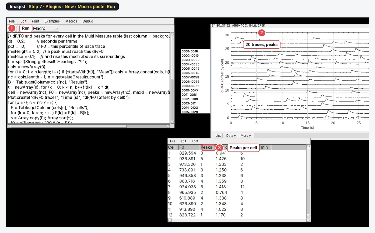
On the worked example below, ImageJ finds 20 cells and 61 calcium transients, 6.1 peaks per minute on average, which is every transient put into the synthetic movie.
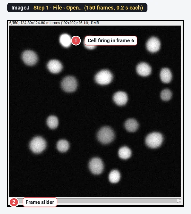
What you need: ImageJ 1.x or Fiji (every command here is in both). A calcium time-lapse (GCaMP, Fluo-4, Cal-520…) as one stack, and the frame interval. The example is a synthetic GCaMP movie (150 frames at 0.2 s, 192 × 192 pixels, 0.65 µm per pixel, 20 cells) made for practice, with every transient at a known frame. Time: about 20 minutes.
What ΔF/F₀ means
Calcium indicators get brighter when calcium rises, but each cell starts at its own brightness: more indicator, a thicker cell, a different focus. ΔF/F₀ removes that by dividing the change by the cell's own resting level. A ΔF/F₀ of 0.5 means 50% brighter than at rest, whatever the cell's starting brightness. The three parts:
How do I measure calcium traces in ImageJ? Step by step
Step 1: Open the movie
Click File › Open… and choose the movie. Step through it: cells flash and fade. Check Image › Properties… for the frame interval (0.2 s here) and the pixel size.
Step 2: Make a Standard Deviation projection
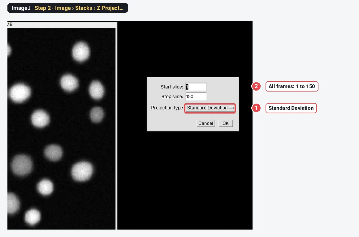
Choose Image › Stacks › Z Project…, keep Start slice 1 and Stop slice 150, set Projection type to Standard Deviation, and click OK. Cells that change over time stand out; anything constant stays dark. (Use Max Intensity or Average Intensity if you also want silent cells.)
Step 3: Threshold the projection
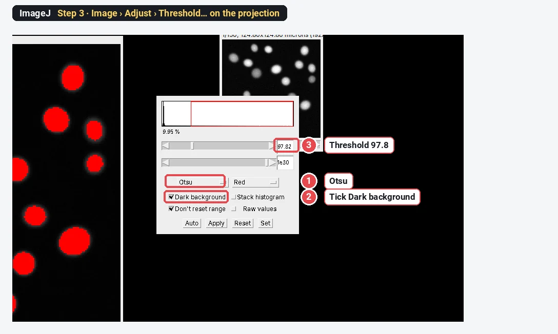
On the projection, choose Image › Adjust › Threshold…, pick Otsu and tick Dark background. Every cell should be red. Click Apply (or Process › Binary › Convert to Mask), then run Process › Binary › Watershed to split cells that touch.
Step 4: Turn the cells into ROIs and add a background ROI
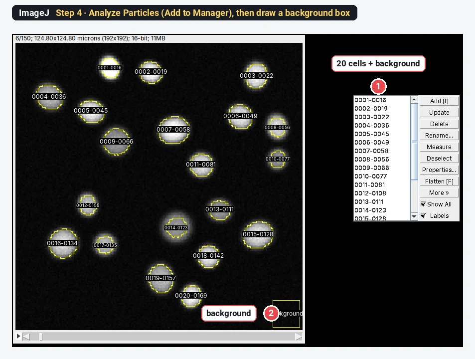
Run Analyze › Analyze Particles… on the mask with a minimum size (20 µm² here), Exclude on edges and Add to Manager. The ROI Manager now lists one ROI per cell: 20 here. Then select the movie, draw a square with the Rectangle tool where there are no cells, press t to add it, and rename it background (it must be the last ROI for the macro below). Drawing cell outlines by hand with the Oval or Freehand tool works too.
Step 5: Look at one cell's trace
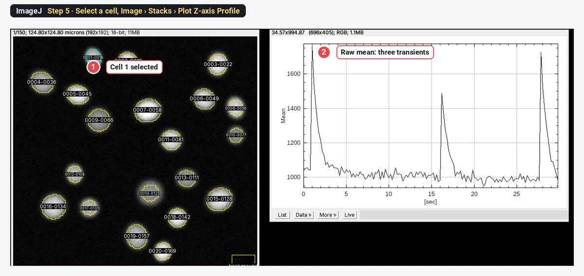
Click one ROI in the ROI Manager and choose Image › Stacks › Plot Z-axis Profile. The plot shows that cell's mean intensity in every frame against time; List gives the numbers. Here the first cell fires three times.
Step 6: Measure all cells with Multi Measure
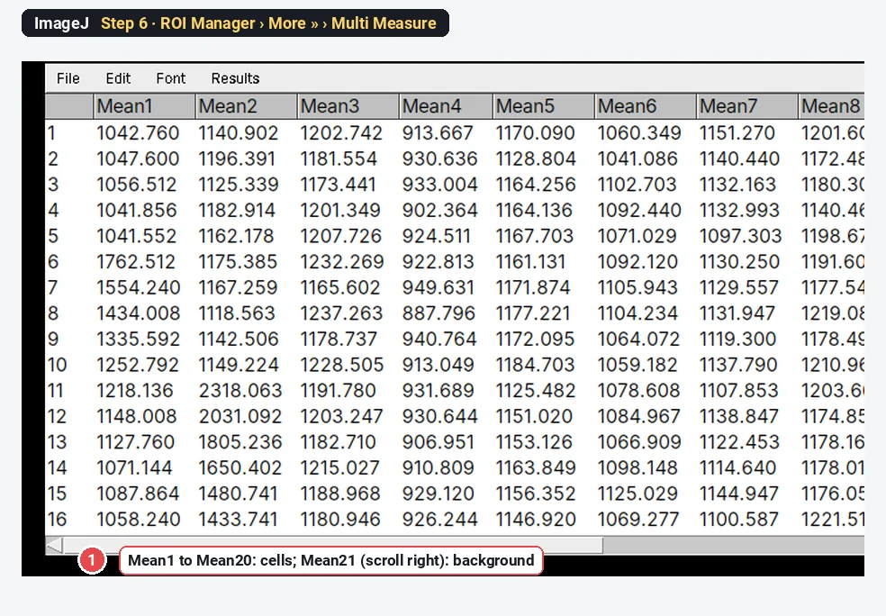
Set Analyze › Set Measurements… to Mean gray value only. In the ROI Manager click Deselect, then More » › Multi Measure, tick Measure all 150 slices and One row per slice, and click OK. The Results table has one row per frame and one column per ROI.
Step 7: Compute ΔF/F₀ and count peaks
Open Plugins › New › Macro, paste the macro below, check the settings at the top and click Run. For each cell it subtracts the background column, takes F₀ as the 10th percentile of the trace, computes ΔF/F₀, finds the peaks, plots all traces one above the other and makes a Peaks table.
// dF/F0 and peaks for every cell in the Multi Measure table (last column = background)
dt = 0.2;         // seconds per frame
pct = 10;         // F0 = this percentile of each trace
minHeight = 0.2;  // a peak must reach this dF/F0
minRise = 0.1;    // and rise this much above its surroundings
h = split(String.getResultsHeadings, "\t");
cols = newArray(0);
for (i = 0; i < h.length; i++) if (startsWith(h[i], "Mean")) cols = Array.concat(cols, h[i]);
nc = cols.length - 1; n = getValue("results.count");
B = Table.getColumn(cols[nc], "Results");
t = newArray(n); for (k = 0; k < n; k++) t[k] = k * dt;
cell = newArray(nc); F0 = newArray(nc); peaks = newArray(nc); maxd = newArray(nc); perMin = newArray(nc);
Plot.create("dF/F0 traces", "Time (s)", "dF/F0 (offset by cell)");
for (c = 0; c < nc; c++) {
  F = Table.getColumn(cols[c], "Results");
  for (k = 0; k < n; k++) F[k] = F[k] - B[k];
  s = Array.copy(F); Array.sort(s);
  f0 = s[floor(pct / 100 * (n - 1))];
  d = newArray(n);
  for (k = 0; k < n; k++) d[k] = (F[k] - f0) / f0;
  p = Array.findMaxima(d, minRise); np = 0;
  for (i = 0; i < p.length; i++) if (d[p[i]] >= minHeight) np++;
  Array.getStatistics(d, mn, mx);
  cell[c] = c + 1; F0[c] = f0; peaks[c] = np; maxd[c] = mx; perMin[c] = np / (n * dt / 60);
  off = newArray(n); for (k = 0; k < n; k++) off[k] = d[k] + 1.5 * (nc - 1 - c);
  Plot.add("line", t, off);
}
Plot.setLimits(0, n * dt, -0.5, 1.5 * nc + 1);
Plot.show();
Table.create("Peaks");
Table.setColumn("Cell", cell); Table.setColumn("F0", F0); Table.setColumn("Peaks", peaks);
Table.setColumn("Max dF/F0", maxd); Table.setColumn("Peaks per min", perMin);
Table.update;Peak counting uses Array.findMaxima(trace, tolerance), a built-in macro function: it returns the maxima that rise more than the tolerance above the trace around them (their prominence). The macro keeps those that also reach ΔF/F₀ ≥ 0.2. Raise minRise if noise gives false peaks; lower it if small events are missed.
The worked example: ΔF/F₀ for one cell
Cell 1, background-subtracted (
| Frame | Time (s) | Raw mean | Background | F | ΔF/F₀ (F₀ = 10th percentile) | ΔF/F₀ (F₀ = frames 1–10) |
|---|---|---|---|---|---|---|
| 1 | 0.0 | 1042.8 | 150.0 | 892.7 | 0.076 | −0.192 |
| 5 | 0.8 | 1041.6 | 153.6 | 888.0 | 0.070 | −0.196 |
| 6 | 1.0 | 1762.5 | 152.6 | 1609.9 | 0.941 | 0.458 |
| 7 | 1.2 | 1554.2 | 154.2 | 1400.0 | 0.688 | 0.268 |
| 8 | 1.4 | 1434.0 | 153.8 | 1280.2 | 0.543 | 0.159 |
| 10 | 1.8 | 1252.8 | 154.0 | 1098.8 | 0.324 | −0.005 |
| 12 | 2.2 | 1148.0 | 155.5 | 992.5 | 0.196 | −0.101 |
| 14 | 2.6 | 1071.1 | 156.0 | 915.1 | 0.103 | −0.171 |
Frame 6, worked through:
All 20 cells, plotted as ΔF/F₀ with the detected peaks marked:
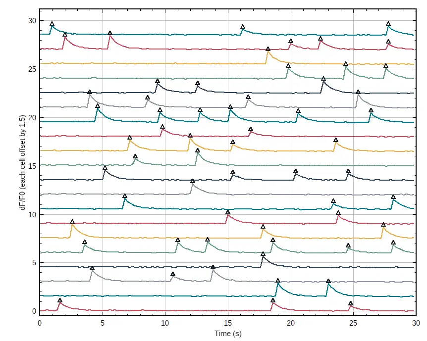
The Peaks table sums to 61 peaks in 20 cells, from 1 to 6 per cell, over 30 s: 6.1 peaks per minute on average. The synthetic movie contains exactly 61 transients, at the frames the macro found.
How do I choose F₀?
F₀ should be the cell at rest. The two common choices:
| F₀ | When it works | When it fails |
|---|---|---|
| Mean of the first N frames (before a stimulus) | Evoked responses with a quiet baseline before the stimulus | Cells that fire during those frames; slow drift over a long recording |
| A low percentile of the whole trace (8th–20th) | Spontaneous activity, no clear quiet period | Cells that are active most of the time (the percentile is no longer rest) |
| A running percentile (a sliding window) | Long recordings with bleaching or drift | Needs a window longer than the events; not a menu command in ImageJ |
On cell 1 the first-frames F₀ includes the transient in frame 6, so it is 33% too high. The whole trace shifts down to −0.19 at rest and the peak halves:
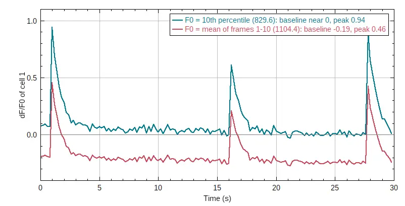
The percentile trace rests a little above zero at the start (0.07) and drifts down: the indicator bleaches slowly during the recording, and the 10th percentile comes from the later frames. For long recordings, correct the bleaching first or use a running baseline.
Pitfalls
- No background subtraction. A camera offset of 100 on a cell at 1,000 shrinks every ΔF/F₀ by about 10%. Always subtract a background ROI frame by frame.
- ROIs bigger than the cells. Dark pixels around the cell dilute F and ΔF. Fit the ROI to the cell; on a standard deviation projection, use a tight threshold.
- Cells that move or drift. Check the ROIs on the last frame; register the stack first if needed.
- Neighbouring cells in one ROI. Two cells in one ROI give a mixed trace. Watershed the mask, or draw ROIs by hand.
- Peaks from noise. Set the rise (prominence) above the noise of the resting trace; check a few cells by eye.
- Comparing ΔF/F₀ across indicators. GCaMP6s, GCaMP6f and dyes have different brightness changes per calcium step; compare like with like.
Reporting it
Calcium imaging was analysed in ImageJ 1.54f. Cells were segmented on a standard-deviation projection (Otsu threshold, watershed, minimum [20] µm²); mean intensities were measured in every frame (ROI Manager, Multi Measure) and background subtracted using a cell-free region. ΔF/F₀ = (F − F₀)/F₀ with F₀ the [10th percentile] of each trace. Peaks were counted with a prominence of [0.1] and a minimum ΔF/F₀ of [0.2]. Values are given as peaks per minute and maximum ΔF/F₀ per cell, [n] cells from [3] experiments.
Cite ImageJ (Schneider et al. 2012); Grienberger and Konnerth (2012) is a good general reference for calcium imaging. Show a few example traces and a raster or summary per condition.
Switch to LabCanvas: ΔF/F₀ traces in a few clicks
LabCanvas Image Analysis has a guided calcium assay in the browser: no macro and no copying columns.
- Open the movie (or click Try it on a sample for the same synthetic recording) and go to Assays › Calcium traces (ΔF/F₀).
- Cells: found on a Standard deviation, Maximum or Mean projection with a threshold, a smallest cell and Split touching cells, or taken from your own ROIs. Background: automatic, none or a region.
- Baseline F₀: a low Percentile of each trace or the first Frames. Peaks: Height ≥, Rise ≥ and Apart ≥.
- Traces: every cell's trace in an interactive chart, a table per cell (F₀, peaks, maximum ΔF/F₀, first peak, frequency, area under the curve), ready to send to Graphs.
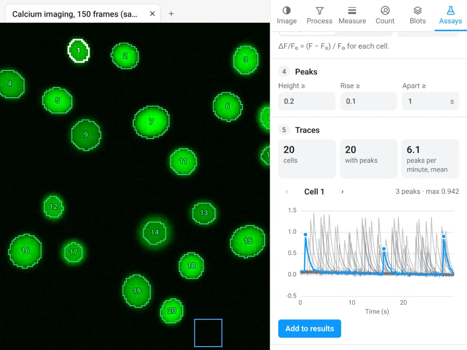
On the same movie LabCanvas finds 20 cells, 20 with peaks, 6.1 peaks per minute on average, the same as the ImageJ macro; for cell 1 the screenshot shows 3 peaks and a maximum ΔF/F₀ of 0.942, against 0.941 in ImageJ.
Why switch for calcium imaging:
- A guided assay instead of a macro: cells, background, F₀ choice and peak settings in one panel, with the trace of the selected cell updating as you change them.
- Every trace and per-cell summary in one table, straight to Graphs for statistics.
- Nothing to install: runs in the browser on any computer or tablet.
Fiji and dedicated tools stay better for large two-photon datasets that need motion correction and neuropil subtraction (Suite2p, CaImAn), and for files in .czi, .nd2 or .lif, which LabCanvas needs as OME-TIFF first.
Open Image Analysis: free with a LabCanvas account (downloading files is part of LabCanvas Pro). ImageJ and Fiji are independent open-source projects; LabCanvas is not affiliated with them.
References
- Grienberger C, Konnerth A (2012). Imaging calcium in neurons. Neuron 73, 862–885. doi:10.1016/j.neuron.2012.02.011
- Schneider CA, Rasband WS, Eliceiri KW (2012). NIH Image to ImageJ: 25 years of image analysis. Nature Methods 9, 671–675. doi:10.1038/nmeth.2089
Frequently asked questions
How do I calculate ΔF/F₀?
How do I choose F₀ for calcium imaging?
Use frames where the cell is at rest. The mean of the first frames works if nothing happens at the start; a low percentile of the whole trace (8th–20th) is safer when cells fire early or spontaneously. On our example, one cell fired in frame 6: with F₀ from frames 1–10 its peak read 0.46 instead of 0.94, and its resting level −0.19.
How do I get a calcium trace in ImageJ?
Select the cell with an ROI and choose Image › Stacks › Plot Z-axis Profile: you get the mean intensity in every frame, with List to copy the numbers. For many cells, add the ROIs to the ROI Manager and use More › Multi Measure with Measure all slices and One row per slice.
Should I subtract background before ΔF/F₀?
Yes. A background offset (camera offset, out-of-focus light) adds to both F and F₀ and shrinks ΔF/F₀. Measure a background region in every frame and subtract it from each cell before computing F₀ and ΔF/F₀.
How do I count calcium peaks in ImageJ?
There is no peak-counting command in the menus, but the macro function Array.findMaxima(trace, tolerance) finds maxima that stand out by more than the tolerance (a prominence). Keep those above a minimum ΔF/F₀ (0.2 here) and count them per cell; divide by the recording time for peaks per minute.
Is there an easier way without installing ImageJ?
LabCanvas Image Analysis has a guided Calcium traces (ΔF/F₀) assay in the browser: it finds the cells, subtracts background, sets F₀, counts peaks and shows every trace. It is free with a LabCanvas account.
Try it in LabCanvas
Every app is free to start in your browser. Create an account and begin.
Start Image Analysis free in your browserKeep reading
ImageJ vs LabCanvas Image Analysis: an honest comparison
ImageJ/Fiji or LabCanvas Image Analysis? Six everyday jobs done in both, six newer ones (macros, vendor files, 3D, StarDist, big images) and which to use.
How to use ImageJ: a beginner's tutorial for the 10 everyday jobs (2026)
How to use ImageJ and Fiji: get started, open an image, then 10 everyday jobs (scale, measure, threshold, count, background, blots) with exact menu paths.
How to set the scale and add a scale bar in ImageJ (with a calibration image to practise on)
Set the scale in ImageJ (Analyze › Set Scale) from a micrometer, scale bar or pixel size, add a scale bar, and practise on a free calibration image.