Graphical abstract template · Graphene research · Characterization
Characterizing graphene
Six measurements tell you what a graphene flake is. Optical contrast on SiO₂/Si finds it, AFM and the Raman spectrum count its layers, the Raman D band gives the distance between its defects, electron diffraction tells one layer from two, and a field-effect device gives its carrier density and mobility.
Updated 10 cited papers46 editable layers

At a glance
- Category
- Graphene research
- Method
- Characterization
- Starting materials
- Exfoliated or CVD graphene on SiO₂/Si (suspended over holes for TEM)
- Product
- Layer number, defect density, crystal structure, carrier density and mobility
- Key result
- Images, spectra and curves computed by LabCanvas from the cited measurements and models; the micrograph’s colours from thin-film optics; the transfer curve’s residual carrier density and contact resistance are illustrative
- Figure
- 1920 × 1080 px (16:9), 46 editable layers, 7 generated objects
Step by step
- Optical contrastOn oxidised silicon, thin-film interference makes a single layer visible; the colours here are computed for graphene with n = 2.6 − 1.3i and 0.34 nm per layer (Blake et al. 2007)
- AFM heightEach layer adds graphite’s interlayer spacing, 0.335 nm; tapping-mode AFM can add as much as 1 nm to the measured height of thin flakes (Nemes-Incze et al. 2008)
- Raman spectrumAt 532 nm a monolayer shows the G band at 1582 cm⁻¹ and one sharp 2D band at 2675 cm⁻¹, about 28 cm⁻¹ wide and 3.6 times as intense; the 2D band changes shape, width and position with the number of layers (Ferrari et al. 2006; Qiu et al. 2016)
- Defect densityI(D)/I(G) against the mean distance between defects, L_D, rises to a maximum near 3 nm and depends on the laser; for L_D ≥ 10 nm, L_D² ≈ 4.3 × 10³ / (E_L⁴ · I(D)/I(G)), with L_D in nm and the laser energy E_L in eV (Cançado et al. 2011)
- Electron diffractionSix-fold spots from the periodicities of 2.13 and 1.23 Å (Meyer et al. 2007); a monolayer’s inner {101̅0} spots are brighter than its outer {112̅0} ones, while in thicker stacks the inner ones are weaker (Hernandez et al. 2008)
- Field effectThe resistance peaks at the Dirac point; on 300 nm SiO₂ each volt on the gate adds 7.2 × 10¹⁰ carriers per cm², and the first devices reached about 10,000 cm²/V·s at room temperature (Novoselov et al. 2004); curve from the model of Kim et al. (2009)
Strengths
- Raman identifies the number of layers without damage and at high throughput (Ferrari et al. 2006)
- The same Raman spectrum also measures the distance between defects (Cançado et al. 2011)
- With monochromatic light graphene can be seen on any SiO₂ thickness; 300 nm and especially about 100 nm suit the eye best (Blake et al. 2007)
Limitations
- AFM heights of thin flakes can be off by as much as 1 nm (Nemes-Incze et al. 2008)
- Visibility depends strongly on the SiO₂ thickness and the wavelength (Blake et al. 2007)
- Electron diffraction needs sheets suspended across holes (Meyer et al. 2007)
Uses
- Quality control of exfoliated, CVD and solution-processed graphene
- Choosing flakes for devices
Papers this template follows
- Ferrari et al., “Raman spectrum of graphene and graphene layers”, Phys. Rev. Lett. 2006. doi:10.1103/PhysRevLett.97.187401primary
- Blake et al., “Making graphene visible”, Appl. Phys. Lett. 2007. doi:10.1063/1.2768624primary
- Cançado et al., “Quantifying defects in graphene via Raman spectroscopy at different excitation energies”, Nano Lett. 2011. doi:10.1021/nl201432gprimary
- Meyer et al., “The structure of suspended graphene sheets”, Nature 2007. doi:10.1038/nature05545primary
- Novoselov et al., “Electric field effect in atomically thin carbon films”, Science 2004. doi:10.1126/science.1102896primary
- Nemes-Incze et al., “Anomalies in thickness measurements of graphene and few layer graphite crystals by tapping mode atomic force microscopy”, Carbon 2008. doi:10.1016/j.carbon.2008.06.022further reading
- Qiu et al., “Raman and conductivity analysis of graphene for biomedical applications”, Materials 2016. doi:10.3390/ma9110897further reading
- Hernandez et al., “High-yield production of graphene by liquid-phase exfoliation of graphite”, Nat. Nanotechnol. 2008. doi:10.1038/nnano.2008.215further reading
- Kim et al., “Realization of a high mobility dual-gated graphene field-effect transistor with Al2O3 dielectric”, Appl. Phys. Lett. 2009. doi:10.1063/1.3077021further reading
- Nair et al., “Fine structure constant defines visual transparency of graphene”, Science 2008. doi:10.1126/science.1156965further reading
Computed by LabCanvas after Ferrari et al., PRL 2006 (doi:10.1103/PhysRevLett.97.187401), Cançado et al., Nano Lett. 2011, Blake et al., APL 2007, Meyer et al., Nature 2007, Novoselov et al., Science 2004, and the papers in the details.
How templates are written and checked: editorial guidelines.
Questions
What does the “Characterizing graphene” template show?
Six measurements tell you what a graphene flake is. Optical contrast on SiO₂/Si finds it, AFM and the Raman spectrum count its layers, the Raman D band gives the distance between its defects, electron diffraction tells one layer from two, and a field-effect device gives its carrier density and mobility.
What are the steps shown in “Characterizing graphene”?
1. Optical contrast: On oxidised silicon, thin-film interference makes a single layer visible; the colours here are computed for graphene with n = 2.6 − 1.3i and 0.34 nm per layer (Blake et al. 2007). 2. AFM height: Each layer adds graphite’s interlayer spacing, 0.335 nm; tapping-mode AFM can add as much as 1 nm to the measured height of thin flakes (Nemes-Incze et al. 2008). 3. Raman spectrum: At 532 nm a monolayer shows the G band at 1582 cm⁻¹ and one sharp 2D band at 2675 cm⁻¹, about 28 cm⁻¹ wide and 3.6 times as intense; the 2D band changes shape, width and position with the number of layers (Ferrari et al. 2006; Qiu et al. 2016). 4. Defect density: I(D)/I(G) against the mean distance between defects, L_D, rises to a maximum near 3 nm and depends on the laser; for L_D ≥ 10 nm, L_D² ≈ 4.3 × 10³ / (E_L⁴ · I(D)/I(G)), with L_D in nm and the laser energy E_L in eV (Cançado et al. 2011). 5. Electron diffraction: Six-fold spots from the periodicities of 2.13 and 1.23 Å (Meyer et al. 2007); a monolayer’s inner {101̅0} spots are brighter than its outer {112̅0} ones, while in thicker stacks the inner ones are weaker (Hernandez et al. 2008). 6. Field effect: The resistance peaks at the Dirac point; on 300 nm SiO₂ each volt on the gate adds 7.2 × 10¹⁰ carriers per cm², and the first devices reached about 10,000 cm²/V·s at room temperature (Novoselov et al. 2004); curve from the model of Kim et al. (2009).
What are the starting materials and the product?
Starting materials: Exfoliated or CVD graphene on SiO₂/Si (suspended over holes for TEM). Product: Layer number, defect density, crystal structure, carrier density and mobility.
Which papers is “Characterizing graphene” based on?
Ferrari et al., “Raman spectrum of graphene and graphene layers”, Phys. Rev. Lett. 2006 (doi:10.1103/PhysRevLett.97.187401); Blake et al., “Making graphene visible”, Appl. Phys. Lett. 2007 (doi:10.1063/1.2768624); Cançado et al., “Quantifying defects in graphene via Raman spectroscopy at different excitation energies”, Nano Lett. 2011 (doi:10.1021/nl201432g); Meyer et al., “The structure of suspended graphene sheets”, Nature 2007 (doi:10.1038/nature05545); Novoselov et al., “Electric field effect in atomically thin carbon films”, Science 2004 (doi:10.1126/science.1102896); Nemes-Incze et al., “Anomalies in thickness measurements of graphene and few layer graphite crystals by tapping mode atomic force microscopy”, Carbon 2008 (doi:10.1016/j.carbon.2008.06.022); Qiu et al., “Raman and conductivity analysis of graphene for biomedical applications”, Materials 2016 (doi:10.3390/ma9110897); Hernandez et al., “High-yield production of graphene by liquid-phase exfoliation of graphite”, Nat. Nanotechnol. 2008 (doi:10.1038/nnano.2008.215); Kim et al., “Realization of a high mobility dual-gated graphene field-effect transistor with Al2O3 dielectric”, Appl. Phys. Lett. 2009 (doi:10.1063/1.3077021); Nair et al., “Fine structure constant defines visual transparency of graphene”, Science 2008 (doi:10.1126/science.1156965).
Can I edit the “Characterizing graphene” template?
Yes. Open it in the LabCanvas editor: all 46 layers are editable, including 7 generated objects (structures, plots, equipment) with their own settings. Change the text, colours and layout, then export PNG, TIFF, SVG or PDF.
Do I need an account to use this template?
Not to view it here. To open and edit it, sign in to LabCanvas or create a free account (the free plan keeps up to 3 designs). Downloading the figure is part of LabCanvas Pro (US$19 a month or US$199 a year).