ΔΔCt method step by step (Livak and Schmittgen 2001)
The 2^−ΔΔCt method step by step: ΔCt, ΔΔCt and fold change with a worked example, the efficiency assumption, the Pfaffl correction and MIQE reference genes.
Contents
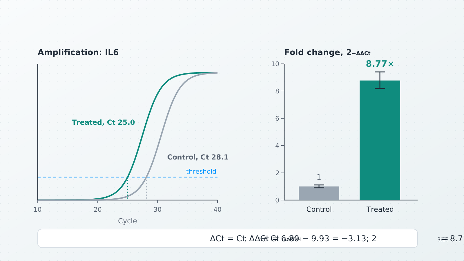
The ΔΔCt method gives the relative expression of a gene from qPCR Ct values: fold change = 2^−ΔΔCt, where ΔCt = Ct(target) − Ct(reference gene) in each sample and ΔΔCt = ΔCt(sample) − ΔCt(control). A ΔΔCt of −3.13 is 2^3.13 = 8.77-fold more expression than in the control. It is the comparative Ct method of Livak and Schmittgen (2001), and it is valid when the target and reference genes amplify with about the same efficiency, close to 100 %.
Below: the formula and where it comes from, a worked example step by step (the same numbers the qPCR ΔΔCt calculator shows when it opens), how to check the efficiency assumption with a standard curve, the Pfaffl correction when efficiencies differ, and how to choose and report reference genes.
The formula
The reference gene (Livak and Schmittgen call it the internal control) corrects for how much RNA went into each reverse transcription. The control (the calibrator) is the sample everything is compared with, such as untreated cells or time zero; its own fold change is 1 by definition.
Why 2? In the exponential phase each cycle multiplies the product by
The MIQE guidelines (Bustin et al. 2009) call the value Cq, the quantification cycle, rather than Ct, Cp or take-off point, which are names different instrument makers gave to the same number. ΔΔCt and ΔΔCq are the same calculation.
Worked example, step by step
IL6 in control and treated cells, with GAPDH as the reference gene, three wells each. Each well holds both assays on the same cDNA, so ΔCt is calculated well by well and then averaged, as Livak and Schmittgen do when target and reference share a well.
| Sample | IL6 Ct | GAPDH Ct | ΔCt |
|---|---|---|---|
| Control | 28.0 | 18.1 | 9.90 |
| Control | 28.3 | 18.2 | 10.10 |
| Control | 28.1 | 18.3 | 9.80 |
| Treated | 25.1 | 18.2 | 6.90 |
| Treated | 24.9 | 18.1 | 6.80 |
| Treated | 25.0 | 18.3 | 6.70 |
- ΔCt in each well: target minus reference. Control: 9.90, 10.10, 9.80. Treated: 6.90, 6.80, 6.70.
- Mean ΔCt per sample: control 9.93 (SD 0.15); treated 6.80 (SD 0.10).
- ΔΔCt: treated minus control,
- Fold change:
- Range: Livak and Schmittgen evaluate
| Sample | Mean ΔCt ± SD | ΔΔCt | Fold change | Range |
|---|---|---|---|---|
| Control | 9.93 ± 0.15 | 0.00 | 1 | 0.90–1.11 |
| Treated | 6.80 ± 0.10 | −3.13 | 8.77 | 8.19–9.40 |
In the calculator. Open the qPCR ΔΔCt calculator: these six wells are its built-in example, and it shows 8.77-fold with this table, a bar chart and a methods sentence to copy. Paste your own Ct values from Excel or the instrument export (one row per well: sample, gene, target Ct, reference Ct) and choose the control sample. Several target genes can go in at once.
In a spreadsheet. With the target Ct in column B and the reference Ct in column C, put =B2-C2 in D2 for ΔCt and fill it down. Average column D for each sample with AVERAGE and subtract the control's average from each sample's average for ΔΔCt; with ΔΔCt in a cell such as F2, =POWER(2,-F2) gives the fold change.
The assumption: equal efficiencies, close to 100 %
The 2^−ΔΔCt formula is only right when both assays double their product every cycle, or at least amplify with the same efficiency. Livak and Schmittgen give two checks.
The validation experiment. Dilute one cDNA over a wide range (they used 100-fold), run target and reference on every dilution, and plot ΔCt against the log of the dilution. If the absolute value of the slope is close to zero, the two efficiencies are similar and ΔΔCt may be used; their example slope was 0.0471. If ΔCt drifts with the dilution, the efficiencies differ: redesign the primers, or use a method that takes the efficiencies into account.
The standard curve. Run a dilution series of each assay alone and plot Ct against log10 of the template amount. MIQE gives the efficiency from the slope of that line:
A slope of −3.32 means an efficiency of 100.1 % (the product doubles each cycle); −3.40 means 96.8 %; −3.10 means 110.2 %. MIQE asks for the calibration curves to be shown to reviewers, for their slopes and y intercepts to be published, and for the linear dynamic range to be stated. The DNA concentration and copy number calculator lays out a qPCR standard dilution series tube by tube.
How much it matters. If the IL6 assay really ran at 90 % while the formula assumes 100 %, the true ratio for the example would be
The Pfaffl correction when efficiencies differ
Pfaffl (2001) puts each assay's own efficiency into the ratio, with
For the example, the mean IL6 Ct falls from 28.13 in the control to 25.00 in treated cells (ΔCt target = 3.13), and the mean GAPDH Ct is 18.20 in both (ΔCt reference = 0.00). With a target efficiency of 95 % (
instead of 8.77. With both efficiencies at 100 % the Pfaffl ratio equals 2^−ΔΔCt. In the calculator, open Primer efficiencies (Pfaffl) and enter 95 and 100: it adds a Pfaffl ratio column and gives 8.11-fold. Enter efficiencies you measured with a standard curve, not guesses.
Reference genes
A reference gene is only useful if its expression does not change with your treatment. Livak and Schmittgen list GAPDH, β-actin, β2-microglobulin and rRNA as suitable internal controls, and highly recommend validating the chosen gene for each experiment. MIQE is firmer: normalisation against a single reference gene is not acceptable unless you present clear evidence that its expression is invariant under your experimental conditions, and the number and choice of reference genes must be determined experimentally and reported. MIQE also asks that they be called reference genes, not housekeeping genes.
- Check stability: the reference gene's Ct should be about the same in every condition when equal amounts of RNA go in. In the example, GAPDH has a mean Ct of 18.20 in both samples.
- Use more than one: Vandesompele et al. (2002) normalise to the geometric mean of several carefully chosen reference genes. In Ct terms, take the mean of the reference genes' Ct values in each well as the reference Ct.
Replicates and statistics
- Technical replicates (repeat wells of one cDNA) measure pipetting and instrument noise: average them first.
- Biological replicates (separate cultures, animals or patients) carry the biological variation, and n is their number. Enter one row per biological replicate (its technical wells averaged), so the SD reflects biology.
- Test ΔCt, report fold change. ΔCt values are close to normally distributed, fold changes are not, so run t tests or ANOVA on ΔCt (or ΔΔCt) and show fold change for readability. Livak and Schmittgen recommend presenting results in the linear form, 2^−ΔΔCt, rather than as raw Ct values.
- Late Cq values: MIQE treats Cq values above 40 as suspect, while warning that any fixed cut-off is arbitrary. Report how you handled very late or undetected wells.
What to report
Among the items the MIQE checklist marks as essential: how the Cq values were determined, the efficiency of each assay calculated from the slope of its calibration curve (with the slope, y intercept and r² of the curve) and its linear dynamic range, the justification of the number and choice of reference genes and a description of the normalisation method, the number of technical replicates (and whether they were reverse-transcription or qPCR replicates), how outliers were identified and handled, the statistical methods and the analysis software; the number of biological replicates is listed as desirable. Name the calculation too: 2^−ΔΔCq (Livak and Schmittgen 2001) or the efficiency-corrected ratio (Pfaffl 2001). The calculator's Copy methods button writes that sentence for you.
Common mistakes
- Averaging fold changes instead of ΔCt values: average on the Ct scale, convert at the end.
- Assuming 100 % efficiency without checking it, or using the Livak formula when a standard curve shows different efficiencies.
- A reference gene that responds to the treatment, which moves every ratio with it.
- Swapping the subtraction: ΔΔCt is sample minus control. Getting it backwards turns an 8.77-fold increase into 0.114.
- Treating technical replicates as biological ones, which makes the SD and any p value far too small.
References
- Livak KJ, Schmittgen TD (2001). Analysis of relative gene expression data using real-time quantitative PCR and the 2^−ΔΔCT method. Methods 25(4), 402–408. doi:10.1006/meth.2001.1262
- Pfaffl MW (2001). A new mathematical model for relative quantification in real-time RT-PCR. Nucleic Acids Research 29(9), e45. doi:10.1093/nar/29.9.e45
- Bustin SA, Benes V, Garson JA, Hellemans J, Huggett J, Kubista M, et al. (2009). The MIQE guidelines: minimum information for publication of quantitative real-time PCR experiments. Clinical Chemistry 55(4), 611–622. doi:10.1373/clinchem.2008.112797
- Vandesompele J, De Preter K, Pattyn F, Poppe B, Van Roy N, De Paepe A, Speleman F (2002). Accurate normalization of real-time quantitative RT-PCR data by geometric averaging of multiple internal control genes. Genome Biology 3(7), research0034. doi:10.1186/gb-2002-3-7-research0034
Frequently asked questions
How do you calculate ΔΔCt?
In each well, subtract the reference-gene Ct from the target Ct (ΔCt). Average the ΔCt values of each sample, then subtract the control's mean ΔCt from the sample's mean ΔCt: that is ΔΔCt. In the worked example, 6.80 − 9.93 = −3.13.
How do I convert ΔΔCt to fold change?
Fold change = 2^−ΔΔCt. A ΔΔCt of −3.13 gives 2^3.13 = 8.77, so the target is expressed about 8.8 times more than in the control. A ΔΔCt of +1 gives 0.5, half the control level.
What are the assumptions of the 2^−ΔΔCt method?
That the target and the reference gene amplify with about the same efficiency, close to 100 % (the product doubles every cycle), and that the reference gene’s expression does not change between your conditions. Livak and Schmittgen check the first with a dilution series: ΔCt should hardly change across the dilutions.
When should I use the Pfaffl method instead of ΔΔCt?
When a standard curve shows that the target and reference efficiencies differ, or are clearly not 100 %. The Pfaffl ratio uses each assay’s measured efficiency: with the target at 95 % and the reference at 100 %, the worked example gives 8.11 instead of 8.77.
How do I calculate PCR efficiency from a standard curve?
Plot Ct against log10 of the template amount for a dilution series and fit a straight line. Efficiency = 10^(−1/slope) − 1 (MIQE). A slope of −3.32 is 100.1 %; −3.40 is 96.8 %.
How many reference genes do I need for qPCR?
The MIQE guidelines say normalisation against a single reference gene is not acceptable unless you show clear evidence that its expression does not change under your experimental conditions, and that the number and choice of reference genes must be determined experimentally. With several reference genes, use the mean of their Ct values as the reference Ct (the geometric mean of their quantities, as in Vandesompele et al. 2002).
Is Ct the same as Cq?
Yes. Cq (quantification cycle) is the name the MIQE guidelines propose for the value instruments call Ct (threshold cycle), Cp (crossing point) or take-off point. The ΔΔCt and ΔΔCq methods are the same calculation.
Try it in LabCanvas
Every app is free to start in your browser. Create an account and begin.
Open the LabCanvas dashboardKeep reading
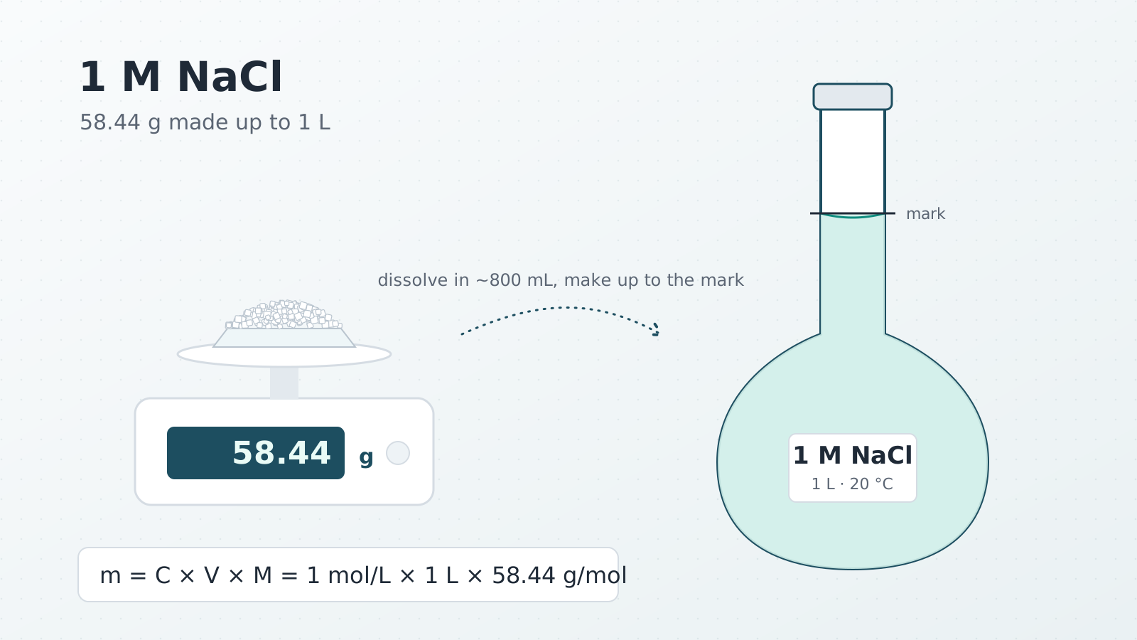
How to make a 1 M NaCl solution (and any molar solution)
Weigh 58.44 g of NaCl, dissolve it in about 800 mL of water and make up to 1 L in a volumetric flask. Molar mass, hydrates, temperature and mistakes.
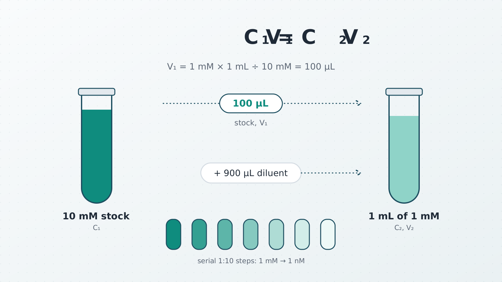
C1V1 = C2V2: the dilution formula with worked examples
C1V1 = C2V2 with worked examples: 10× buffer to 1×, a 1:1000 antibody, serial dilutions, consistent units, and when the dilution formula does not apply.
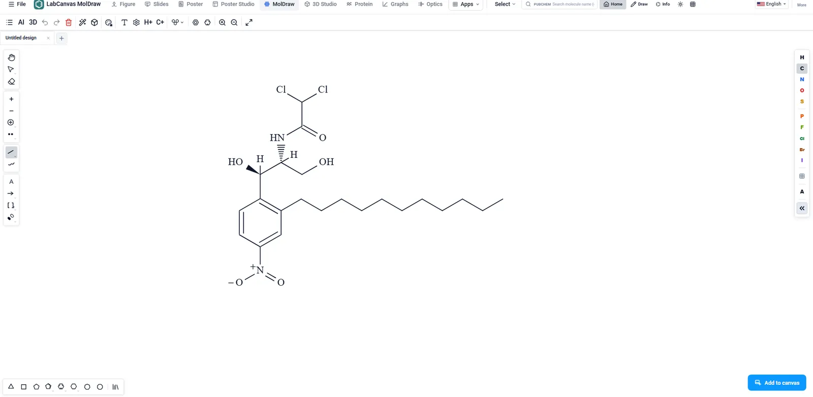
ChemDraw vs LabCanvas MolDraw: chemical structure drawing compared
ChemDraw or LabCanvas MolDraw? Drawing, names, NMR, file formats, price and platforms side by side, a reaction-scheme example, and when ChemDraw is better.