CircuiTikZ: drawing circuits in LaTeX
Quick answer
\usepackage{circuitikz} (it loads TikZ) and draw inside \begin{circuitikz} … \end{circuitikz}. Two-terminal components sit on a path: \draw (0,0) to[R=$R_1$] (2,0); draws a resistor labelled R1 between the two points, to[C], to[L], to[V], to[battery1] or to[spst] work the same way, and -- is plain wire. Parts with more pins (op-amps, transistors, logic gates, ground) are nodes, placed with node[op amp] (OA) {} and wired through anchors such as (OA.out). Package options choose the symbols: \usepackage[american]{circuitikz} or [european].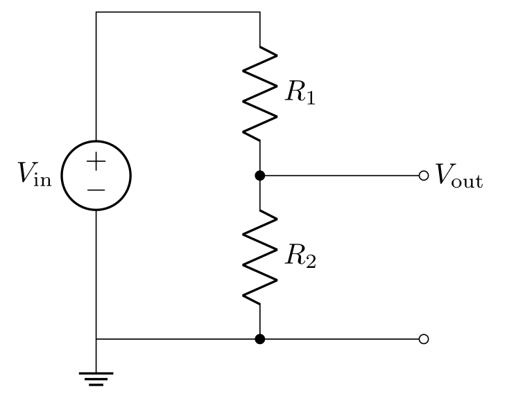
\usepackage{tikz} \usepackage[american, RPvoltages]{circuitikz}\begin{circuitikz}
\draw (0,0) to[V, l=$V_\mathrm{in}$] (0,4)
-- (2,4) to[R, l=$R_1$] (2,2)
to[R, l=$R_2$] (2,0) -- (0,0);
\draw (2,2) to[short, *-o] (4,2) node[right] {$V_\mathrm{out}$};
\draw (2,0) to[short, *-o] (4,0);
\draw (0,0) node[ground] {};
\end{circuitikz}Full document
\documentclass[border=4pt]{standalone}
\usepackage{tikz}
\usepackage[american, RPvoltages]{circuitikz}
\begin{document}
\begin{circuitikz}
  \draw (0,0) to[V, l=$V_\mathrm{in}$] (0,4)
        -- (2,4) to[R, l=$R_1$] (2,2)
        to[R, l=$R_2$] (2,0) -- (0,0);
  \draw (2,2) to[short, *-o] (4,2) node[right] {$V_\mathrm{out}$};
  \draw (2,0) to[short, *-o] (4,0);
  \draw (0,0) node[ground] {};
\end{circuitikz}
\end{document}Contents
Loading CircuiTikZ: package options and styles
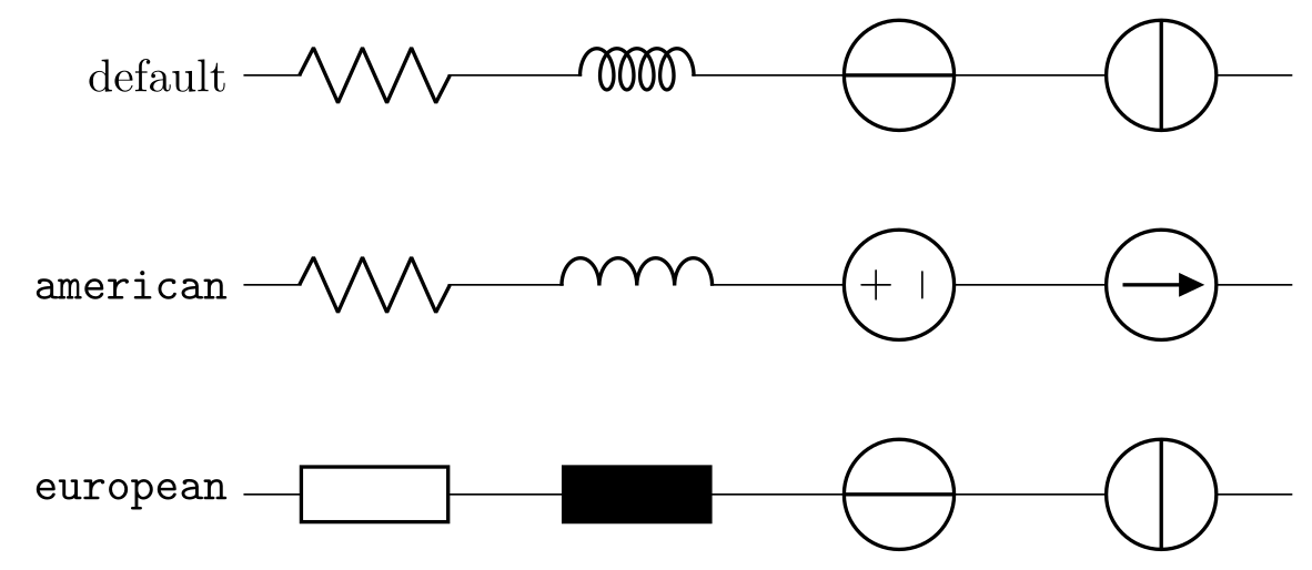
CircuiTikZ (current version 1.8.7 of 2026-09-12, included in TeX Live and MiKTeX) loads TikZ and the TikZ libraries calc, arrows.meta, bending and fpu. The circuitikz environment is an alias of tikzpicture, so all TikZ commands work inside it. Without options you get a mix: American zig-zag resistors and logic ports, “cute” curly inductors, and European voltage and current sources. The options that matter, as named in the manual:
| Option | Effect |
|---|---|
american | American currents, voltages (+/− signs), resistors (zig-zag), inductors (bumps), ports and surge arresters |
european | The European versions of all of these: rectangle resistors, filled-rectangle inductors, voltage arrows, rectangular logic ports |
RPvoltages, EFvoltages | Direction of voltages: arrows towards rising potential (RP) or along the electric field (EF). The default is the older nooldvoltagedirection; the manual advises choosing one explicitly |
siunitx | Lets labels written 2<\ohm> mean \SI{2}{\ohm}. Marked experimental; the maintainers suggest plain \qty{2}{\ohm} from siunitx instead |
americanresistors, europeanresistors, cuteinductors, americaninductors, europeaninductors, americanvoltages, europeanvoltages, straightvoltages, americancurrents, europeancurrents, americanports, europeanports | One family at a time |
smartlabels (default), rotatelabels, straightlabels | Whether labels turn with the component |
The same names work as styles for one circuit or scope, \begin{circuitikz}[european], so one document can mix them. Every example on this page that has voltage signs uses [american, RPvoltages].
\usepackage{tikz} \usepackage{circuitikz}\begin{circuitikz}
% the same code, R, L, V and I, in three styles
\draw (0,0) node[left] {default} to[R] ++(2,0) to[L] ++(2,0) to[V] ++(2,0) to[I] ++(2,0);
\begin{scope}[american, yshift=-1.6cm]
\draw (0,0) node[left] {\texttt{american}} to[R] ++(2,0) to[L] ++(2,0) to[V] ++(2,0) to[I] ++(2,0);
\end{scope}
\begin{scope}[european, yshift=-3.2cm]
\draw (0,0) node[left] {\texttt{european}} to[R] ++(2,0) to[L] ++(2,0) to[V] ++(2,0) to[I] ++(2,0);
\end{scope}
\end{circuitikz}Full document
\documentclass[border=4pt]{standalone}
\usepackage{tikz}
\usepackage{circuitikz}
\begin{document}
\begin{circuitikz}
  % the same code, R, L, V and I, in three styles
  \draw (0,0) node[left] {default} to[R] ++(2,0) to[L] ++(2,0) to[V] ++(2,0) to[I] ++(2,0);
  \begin{scope}[american, yshift=-1.6cm]
    \draw (0,0) node[left] {\texttt{american}} to[R] ++(2,0) to[L] ++(2,0) to[V] ++(2,0) to[I] ++(2,0);
  \end{scope}
  \begin{scope}[european, yshift=-3.2cm]
    \draw (0,0) node[left] {\texttt{european}} to[R] ++(2,0) to[L] ++(2,0) to[V] ++(2,0) to[I] ++(2,0);
  \end{scope}
\end{circuitikz}
\end{document}The to[ ] syntax: components on a path
Two-terminal (“path-style”) components are drawn with TikZ’s to operation: (a) to[⟨component⟩, ⟨options⟩] (b) places the component in the middle of the segment from a to b and fills the rest with wire. The component itself keeps its size (bipoles/length, 1.4 cm by default), so a longer segment just means longer leads; \ctikzset{bipoles/length=.8cm} makes every component smaller.
to[R=$R_1$]is short forto[R, l=$R_1$]on passive parts; on a voltage source it sets the voltagev=, on a current source the currenti=.to[short]is a wire that can carry labels and poles,to[open]draws nothing but can carry a voltage.- The direction of the path matters: labels are placed relative to it, and the polarity of sources and diodes follows it. To change a component’s orientation use
invertandmirror, neverxscale=-1oryscale=-1(the manual warns that they mess up the path);invertis the one that swaps the + and − of a source. name=D1(orn=D1) names a component, so you can connect to its anchors later.
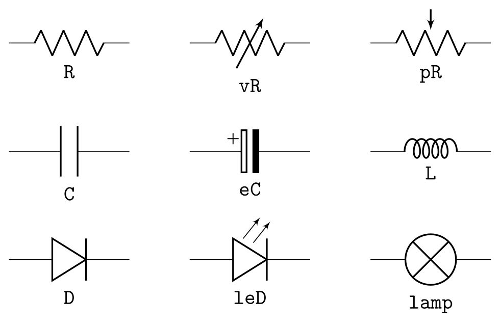
Names are case-sensitive and short: R, vR (variable), pR (potentiometer), C, eC (electrolytic), L, D, leD (LED), lamp, fuse; chapter 4 of the manual lists every one with its aliases and anchors.
\usepackage{tikz} \usepackage{circuitikz}\begin{circuitikz}
\draw (0,0) to[R, l_=\texttt{R}] ++(2,0);
\draw (3,0) to[vR, l_=\texttt{vR}] ++(2,0);
\draw (6,0) to[pR, l_=\texttt{pR}] ++(2,0);
\draw (0,-1.8) to[C, l_=\texttt{C}] ++(2,0);
\draw (3,-1.8) to[eC, l_=\texttt{eC}] ++(2,0);
\draw (6,-1.8) to[L, l_=\texttt{L}] ++(2,0);
\draw (0,-3.6) to[D, l_=\texttt{D}] ++(2,0);
\draw (3,-3.6) to[leD, l_=\texttt{leD}] ++(2,0);
\draw (6,-3.6) to[lamp, l_=\texttt{lamp}] ++(2,0);
\end{circuitikz}Full document
\documentclass[border=4pt]{standalone}
\usepackage{tikz}
\usepackage{circuitikz}
\begin{document}
\begin{circuitikz}
  \draw (0,0)    to[R, l_=\texttt{R}]       ++(2,0);
  \draw (3,0)    to[vR, l_=\texttt{vR}]     ++(2,0);
  \draw (6,0)    to[pR, l_=\texttt{pR}]     ++(2,0);
  \draw (0,-1.8) to[C, l_=\texttt{C}]       ++(2,0);
  \draw (3,-1.8) to[eC, l_=\texttt{eC}]     ++(2,0);
  \draw (6,-1.8) to[L, l_=\texttt{L}]       ++(2,0);
  \draw (0,-3.6) to[D, l_=\texttt{D}]       ++(2,0);
  \draw (3,-3.6) to[leD, l_=\texttt{leD}]   ++(2,0);
  \draw (6,-3.6) to[lamp, l_=\texttt{lamp}] ++(2,0);
\end{circuitikz}
\end{document}Voltage and current sources
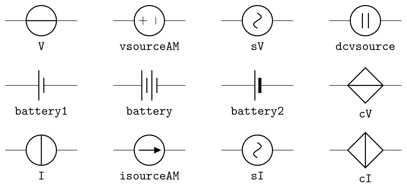
V (also vsource) and I (isource) follow the chosen style: a circle crossed along the wire (European voltage), across it (European current), +/− signs or an arrow (American). To get one style whatever the options, use the explicit names vsourceAM and isourceAM (American) or vsourceEU and isourceEU (European). Also available: sV and sI (sinusoidal), dcvsource and dcisource, the batteries battery1 (one cell), battery (two cells) and battery2, and the controlled (dependent) sources cV and cI, drawn as diamonds.
Polarity. Where the + of a source or the long plate of a battery ends up depends on the direction you draw it and on the voltage-direction option. With RPvoltages the + is at the end of the path, so a source drawn upwards from ground, (0,0) to[V] (0,4), has its + on top, as in the voltage divider above. With the default nooldvoltagedirection the same code puts the + at the bottom (the catalogue below uses the default options). Add invert to turn one source round.
\usepackage{tikz} \usepackage{circuitikz}\begin{circuitikz}
\draw (0,0) to[V, l_=\texttt{V}] ++(2,0);
\draw (3,0) to[vsourceAM, l_=\texttt{vsourceAM}] ++(2,0);
\draw (6,0) to[sV, l_=\texttt{sV}] ++(2,0);
\draw (9,0) to[dcvsource, l_=\texttt{dcvsource}] ++(2,0);
\draw (0,-1.8) to[battery1, l_=\texttt{battery1}] ++(2,0);
\draw (3,-1.8) to[battery, l_=\texttt{battery}] ++(2,0);
\draw (6,-1.8) to[battery2, l_=\texttt{battery2}] ++(2,0);
\draw (9,-1.8) to[cV, l_=\texttt{cV}] ++(2,0);
\draw (0,-3.6) to[I, l_=\texttt{I}] ++(2,0);
\draw (3,-3.6) to[isourceAM, l_=\texttt{isourceAM}] ++(2,0);
\draw (6,-3.6) to[sI, l_=\texttt{sI}] ++(2,0);
\draw (9,-3.6) to[cI, l_=\texttt{cI}] ++(2,0);
\end{circuitikz}Full document
\documentclass[border=4pt]{standalone}
\usepackage{tikz}
\usepackage{circuitikz}
\begin{document}
\begin{circuitikz}
  \draw (0,0)    to[V, l_=\texttt{V}]                 ++(2,0);
  \draw (3,0)    to[vsourceAM, l_=\texttt{vsourceAM}] ++(2,0);
  \draw (6,0)    to[sV, l_=\texttt{sV}]               ++(2,0);
  \draw (9,0)    to[dcvsource, l_=\texttt{dcvsource}] ++(2,0);
  \draw (0,-1.8) to[battery1, l_=\texttt{battery1}]   ++(2,0);
  \draw (3,-1.8) to[battery, l_=\texttt{battery}]     ++(2,0);
  \draw (6,-1.8) to[battery2, l_=\texttt{battery2}]   ++(2,0);
  \draw (9,-1.8) to[cV, l_=\texttt{cV}]               ++(2,0);
  \draw (0,-3.6) to[I, l_=\texttt{I}]                 ++(2,0);
  \draw (3,-3.6) to[isourceAM, l_=\texttt{isourceAM}] ++(2,0);
  \draw (6,-3.6) to[sI, l_=\texttt{sI}]               ++(2,0);
  \draw (9,-3.6) to[cI, l_=\texttt{cI}]               ++(2,0);
\end{circuitikz}
\end{document}Switches and push buttons
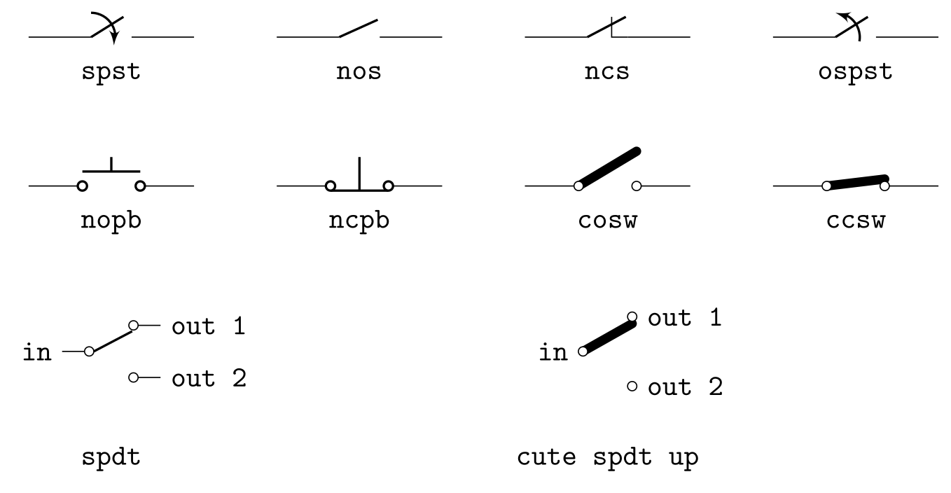
spst(alias ofswitch) is drawn as a closing switch with an arrow, the same symbol ascspst;ospstis the opening switch. For the plain symbols usenos(normally open) andncs(normally closed);cnos,onos,cncs,oncsadd the closing/opening arrow.- Push buttons:
nopb(orpush button),ncpb, andnopbc/ncpbofor the same buttons drawn in their operated position. - “Cute” switches with round contacts:
cosw(open),ccsw(closed),cogsw/ccgsw(opening/closing). - Single-pole double-throw switches are nodes:
node[spdt] (S) {}with anchorsS.in,S.out 1,S.out 2, orcute spdt up,cute spdt mid,cute spdt down. There is also a path-styletoggle switch, rotary switches and jumpers.
\usepackage{tikz} \usepackage{circuitikz}\begin{circuitikz}
\draw (0,0) to[spst, l_=\texttt{spst}] ++(2,0);
\draw (3,0) to[nos, l_=\texttt{nos}] ++(2,0);
\draw (6,0) to[ncs, l_=\texttt{ncs}] ++(2,0);
\draw (9,0) to[ospst, l_=\texttt{ospst}] ++(2,0);
\draw (0,-1.8) to[nopb, l_=\texttt{nopb}] ++(2,0);
\draw (3,-1.8) to[ncpb, l_=\texttt{ncpb}] ++(2,0);
\draw (6,-1.8) to[cosw, l_=\texttt{cosw}] ++(2,0);
\draw (9,-1.8) to[ccsw, l_=\texttt{ccsw}] ++(2,0);
% single-pole double-throw switches are nodes with anchors
\draw (1,-3.8) node[spdt] (S) {} (S.in) node[left] {\texttt{in}}
(S.out 1) node[right] {\texttt{out 1}} (S.out 2) node[right] {\texttt{out 2}};
\node at (1,-5.1) {\texttt{spdt}};
\draw (7,-3.8) node[cute spdt up] (T) {} (T.in) node[left] {\texttt{in}}
(T.out 1) node[right] {\texttt{out 1}} (T.out 2) node[right] {\texttt{out 2}};
\node at (7,-5.1) {\texttt{cute spdt up}};
\end{circuitikz}Full document
\documentclass[border=4pt]{standalone}
\usepackage{tikz}
\usepackage{circuitikz}
\begin{document}
\begin{circuitikz}
  \draw (0,0)    to[spst, l_=\texttt{spst}]       ++(2,0);
  \draw (3,0)    to[nos, l_=\texttt{nos}]         ++(2,0);
  \draw (6,0)    to[ncs, l_=\texttt{ncs}]         ++(2,0);
  \draw (9,0)    to[ospst, l_=\texttt{ospst}]     ++(2,0);
  \draw (0,-1.8) to[nopb, l_=\texttt{nopb}]       ++(2,0);
  \draw (3,-1.8) to[ncpb, l_=\texttt{ncpb}]       ++(2,0);
  \draw (6,-1.8) to[cosw, l_=\texttt{cosw}]       ++(2,0);
  \draw (9,-1.8) to[ccsw, l_=\texttt{ccsw}]       ++(2,0);
  % single-pole double-throw switches are nodes with anchors
  \draw (1,-3.8) node[spdt] (S) {} (S.in) node[left] {\texttt{in}}
        (S.out 1) node[right] {\texttt{out 1}} (S.out 2) node[right] {\texttt{out 2}};
  \node at (1,-5.1) {\texttt{spdt}};
  \draw (7,-3.8) node[cute spdt up] (T) {} (T.in) node[left] {\texttt{in}}
        (T.out 1) node[right] {\texttt{out 1}} (T.out 2) node[right] {\texttt{out 2}};
  \node at (7,-5.1) {\texttt{cute spdt up}};
\end{circuitikz}
\end{document}Labels, annotations, voltages and currents
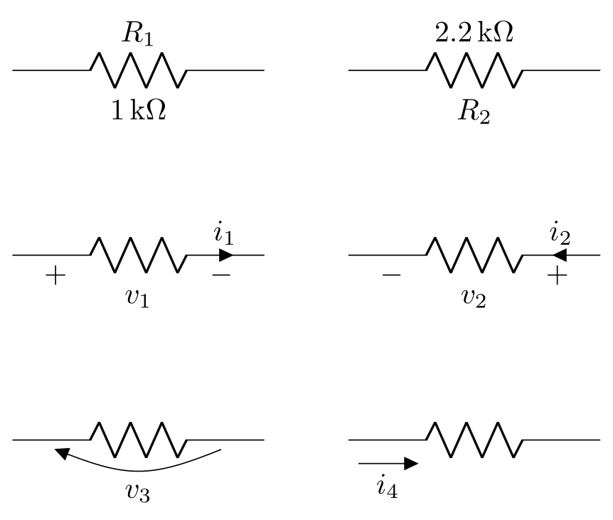
Every path-style component takes these keys; _ or ^ after the key puts the text below or above (relative to the drawing direction):
| Key | Draws |
|---|---|
l= | Label, above by default (the name, e.g. $R_1$) |
a= | Annotation, below by default (the value) |
v= | Voltage: +/− signs with American voltages, a curved arrow with European ones (straight voltages and raised voltages are the other styles); v<= / v>= reverse it |
i= | Current arrow on the wire: i_>, i^<, i>_… choose side (^ _) and direction (> <); the order of the two characters picks the lead before or after the component |
f= | Flow arrow beside the wire, with the same modifiers |
The default direction of v and i differs between passive parts and sources and depends on the voltage-direction option, so check the first circuit you draw. Labels that contain = or , must be braced, to[R={$R_1=10\,\Omega$}], or the option parser splits them. l2=… and … stacks a label on two lines. For the voltage between two terminals that are not joined by a component, draw to[open, v=…] between them, as in the RC filter below.
\usepackage{tikz} \usepackage[american, RPvoltages]{circuitikz}\begin{circuitikz}
% l = label, a = annotation; _ and ^ choose the side
\draw (0,0) to[R, l=$R_1$, a=$1\,\mathrm{k\Omega}$] ++(3,0);
\draw (4,0) to[R, l_=$R_2$, a^=$2.2\,\mathrm{k\Omega}$] ++(3,0);
% v = voltage, i = current; > or < reverses the default direction
\draw (0,-2.2) to[R, v=$v_1$, i=$i_1$] ++(3,0);
\draw (4,-2.2) to[R, v>=$v_2$, i^<=$i_2$] ++(3,0);
% european-style voltage arrow and a flow arrow f
\begin{scope}[european voltages, yshift=-4.4cm]
\draw (0,0) to[R, v=$v_3$] ++(3,0);
\draw (4,0) to[R, f>_=$i_4$] ++(3,0);
\end{scope}
\end{circuitikz}Full document
\documentclass[border=4pt]{standalone}
\usepackage{tikz}
\usepackage[american, RPvoltages]{circuitikz}
\begin{document}
\begin{circuitikz}
  % l = label, a = annotation; _ and ^ choose the side
  \draw (0,0) to[R, l=$R_1$, a=$1\,\mathrm{k\Omega}$] ++(3,0);
  \draw (4,0) to[R, l_=$R_2$, a^=$2.2\,\mathrm{k\Omega}$] ++(3,0);
  % v = voltage, i = current; > or < reverses the default direction
  \draw (0,-2.2) to[R, v=$v_1$, i=$i_1$] ++(3,0);
  \draw (4,-2.2) to[R, v>=$v_2$, i^<=$i_2$] ++(3,0);
  % european-style voltage arrow and a flow arrow f
  \begin{scope}[european voltages, yshift=-4.4cm]
    \draw (0,0) to[R, v=$v_3$] ++(3,0);
    \draw (4,0) to[R, f>_=$i_4$] ++(3,0);
  \end{scope}
\end{circuitikz}
\end{document}Poles (connection dots) and ground
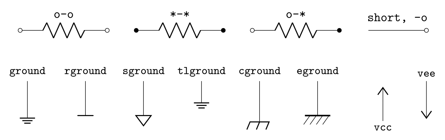
The pole shortcuts go in the options of a component or a short: * is a filled dot (a junction), o an open circle (a terminal), d a diamond; -* puts one at the end only, o- at the start, *-o both. The general form is bipole nodes={circ}{ocirc}. Poles are added after the path is drawn and open ones are filled white, so draw a pole in the same \draw as the wires it covers. A dot on its own is node[circ] {}.
Grounds and supply rails are nodes whose anchor is the connection point: node[ground] {}, rground, sground (signal), tlground (tailless), tground, nground, pground (protective), cground (chassis), eground and eground2 (European); vcc and vee for supply arrows.
\usepackage{tikz} \usepackage{circuitikz}\begin{circuitikz}
% poles at the ends of a component: o open, * filled, d diamond
\draw (0,0) to[R, o-o, l=\texttt{o-o}] ++(2.4,0);
\draw (3.2,0) to[R, *-*, l=\texttt{*-*}] ++(2.4,0);
\draw (6.4,0) to[R, o-*, l=\texttt{o-*}] ++(2.4,0);
\draw (9.6,0) to[short, -o, l=\texttt{short, -o}] ++(1.6,0);
% grounds and supply rails are nodes: their anchor is where the wire connects
\foreach \s [count=\i] in {ground, rground, sground, tlground, cground, eground} {
\draw (1.6*\i-1.4,-1.4) node[above, font=\ttfamily\small] {\s} -- ++(0,-0.6) node[\s] {};
}
\draw (10,-2) node[vcc] {} -- ++(0,-0.5) node[below, font=\ttfamily\small] {vcc};
\draw (11.2,-1.4) -- ++(0,-0.6) node[vee] {};
\node[above, font=\ttfamily\small] at (11.2,-1.4) {vee};
\end{circuitikz}Full document
\documentclass[border=4pt]{standalone}
\usepackage{tikz}
\usepackage{circuitikz}
\begin{document}
\begin{circuitikz}
  % poles at the ends of a component: o open, * filled, d diamond
  \draw (0,0) to[R, o-o, l=\texttt{o-o}] ++(2.4,0);
  \draw (3.2,0) to[R, *-*, l=\texttt{*-*}] ++(2.4,0);
  \draw (6.4,0) to[R, o-*, l=\texttt{o-*}] ++(2.4,0);
  \draw (9.6,0) to[short, -o, l=\texttt{short, -o}] ++(1.6,0);
  % grounds and supply rails are nodes: their anchor is where the wire connects
  \foreach \s [count=\i] in {ground, rground, sground, tlground, cground, eground} {
    \draw (1.6*\i-1.4,-1.4) node[above, font=\ttfamily\small] {\s} -- ++(0,-0.6) node[\s] {};
  }
  \draw (10,-2) node[vcc] {} -- ++(0,-0.5) node[below, font=\ttfamily\small] {vcc};
  \draw (11.2,-1.4) -- ++(0,-0.6) node[vee] {};
  \node[above, font=\ttfamily\small] at (11.2,-1.4) {vee};
\end{circuitikz}
\end{document}Op-amps
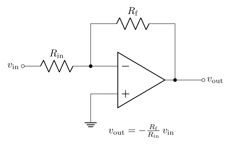
node[op amp] (OA) {} draws an operational amplifier with the anchors OA.- (inverting input), OA.+, OA.out, and OA.up / OA.down for the supplies. The inverting input is on top by default; noinv input up swaps the inputs. Other amplifiers: en amp (DIN/EN 60617 box), fd op amp (fully differential), inst amp, gm amp, plain amp, buffer.
In the inverting amplifier below, the input resistor ends at a coordinate (J) (a named point, not a node, so wires join without gaps) and (T -| OA.out) is the point above the output: x of OA.out, y of T.
\usepackage{tikz} \usepackage[american, RPvoltages]{circuitikz}\begin{circuitikz}
% op amp node: anchors -, + and out (the inverting input is on top)
\draw (0,0) node[op amp] (OA) {};
\draw (OA.-) ++(-3,0) node[left] {$v_\mathrm{in}$}
to[R, l=$R_\mathrm{in}$, o-*] ++(2.4,0) coordinate (J) -- (OA.-);
\draw (J) -- ++(0,1.5) coordinate (T)
to[R, l=$R_\mathrm{f}$] (T -| OA.out) -- (OA.out);
\draw (OA.out) to[short, *-o] ++(1,0) node[right] {$v_\mathrm{out}$};
\draw (OA.+) -- ++(-0.6,0) -- ++(0,-0.6) node[ground] {};
\node at (0,-1.8) {$v_\mathrm{out} = -\frac{R_\mathrm{f}}{R_\mathrm{in}}\,v_\mathrm{in}$};
\end{circuitikz}Full document
\documentclass[border=4pt]{standalone}
\usepackage{tikz}
\usepackage[american, RPvoltages]{circuitikz}
\begin{document}
\begin{circuitikz}
  % op amp node: anchors -, + and out (the inverting input is on top)
  \draw (0,0) node[op amp] (OA) {};
  \draw (OA.-) ++(-3,0) node[left] {$v_\mathrm{in}$}
        to[R, l=$R_\mathrm{in}$, o-*] ++(2.4,0) coordinate (J) -- (OA.-);
  \draw (J) -- ++(0,1.5) coordinate (T)
        to[R, l=$R_\mathrm{f}$] (T -| OA.out) -- (OA.out);
  \draw (OA.out) to[short, *-o] ++(1,0) node[right] {$v_\mathrm{out}$};
  \draw (OA.+) -- ++(-0.6,0) -- ++(0,-0.6) node[ground] {};
  \node at (0,-1.8) {$v_\mathrm{out} = -\frac{R_\mathrm{f}}{R_\mathrm{in}}\,v_\mathrm{in}$};
\end{circuitikz}
\end{document}Transistors
Transistors are nodes. Bipolar npn and pnp have the anchors B, C, E (or base, collector, emitter); nmos, pmos, nfet, pfet, nigfete and the other MOSFETs have G, D, S (gate, drain, source), njfet / pjfet also have G, D, S, and nigbt / pigbt have B, C, E. Put a T in front to use one on a path, to[Tnmos], with the gate at right angles to the path. Package options such as arrowmos and fetbodydiode change the MOSFET symbols.
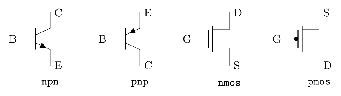
\usepackage{tikz} \usepackage{circuitikz}\begin{circuitikz}[font=\small]
\foreach \t/\x in {npn/0, pnp/2.6} {
\draw (\x,0) node[\t] (Q) {}
(Q.B) node[left] {B} (Q.C) node[right] {C} (Q.E) node[right] {E};
\node at (\x,-1.3) {\texttt{\t}};
}
\foreach \t/\x in {nmos/5.2, pmos/7.8} {
\draw (\x,0) node[\t] (M) {}
(M.G) node[left] {G} (M.D) node[right] {D} (M.S) node[right] {S};
\node at (\x,-1.3) {\texttt{\t}};
}
\end{circuitikz}Full document
\documentclass[border=4pt]{standalone}
\usepackage{tikz}
\usepackage{circuitikz}
\begin{document}
\begin{circuitikz}[font=\small]
  \foreach \t/\x in {npn/0, pnp/2.6} {
    \draw (\x,0) node[\t] (Q) {}
      (Q.B) node[left] {B} (Q.C) node[right] {C} (Q.E) node[right] {E};
    \node at (\x,-1.3) {\texttt{\t}};
  }
  \foreach \t/\x in {nmos/5.2, pmos/7.8} {
    \draw (\x,0) node[\t] (M) {}
      (M.G) node[left] {G} (M.D) node[right] {D} (M.S) node[right] {S};
    \node at (\x,-1.3) {\texttt{\t}};
  }
\end{circuitikz}
\end{document}Logic gates: American, European and IEEE ports
Logic gates are nodes named and port, or port, nand port, nor port, xor port, xnor port, not port and buffer port, with the anchors in 1, in 2 (more with number inputs=4) and out. By default they use the legacy American shapes; the europeanports option gives the rectangular IEC ones. Since version 1.1.0 there is also a set drawn to the proportions of IEEE Std 91a-1991: write ieeestd and port, or set \ctikzset{logic ports=ieee} to make and port mean the IEEE shape. IEEE gates keep their proportions when resized and are sized to line up with the chip components; placed with anchor=in 1 they stack neatly, as in the half adder further down.
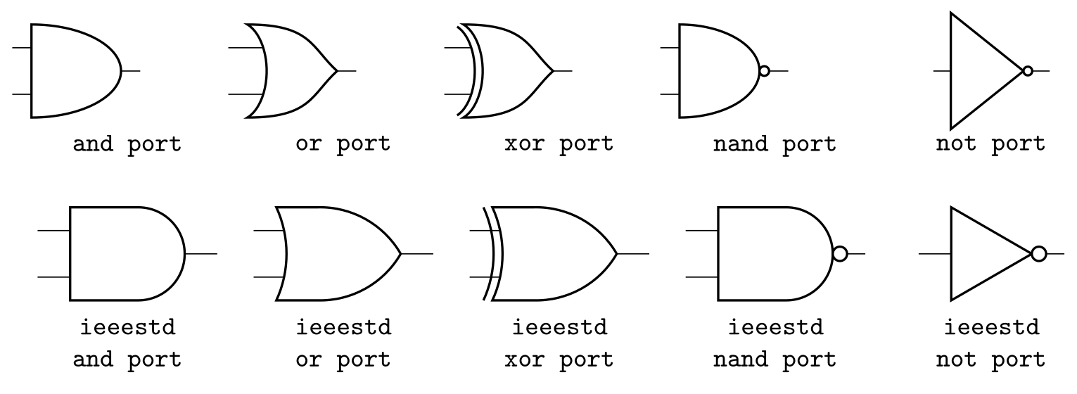
\usepackage{tikz} \usepackage{circuitikz}\begin{circuitikz}[font=\small\ttfamily]
\foreach \p [count=\i] in {and port, or port, xor port, nand port, not port} {
% legacy (american) shapes: the default
\node[\p] at (2.6*\i,0) {};
\node at (2.6*\i,-0.9) {\p};
% IEEE Std 91a shapes: prefix ieeestd (or \ctikzset{logic ports=ieee})
\node[ieeestd \p] at (2.6*\i,-2.2) {};
\node[align=center] at (2.6*\i,-3.3) {ieeestd\\\p};
}
\end{circuitikz}Full document
\documentclass[border=4pt]{standalone}
\usepackage{tikz}
\usepackage{circuitikz}
\begin{document}
\begin{circuitikz}[font=\small\ttfamily]
  \foreach \p [count=\i] in {and port, or port, xor port, nand port, not port} {
    % legacy (american) shapes: the default
    \node[\p] at (2.6*\i,0) {};
    \node at (2.6*\i,-0.9) {\p};
    % IEEE Std 91a shapes: prefix ieeestd (or \ctikzset{logic ports=ieee})
    \node[ieeestd \p] at (2.6*\i,-2.2) {};
    \node[align=center] at (2.6*\i,-3.3) {ieeestd\\\p};
  }
\end{circuitikz}
\end{document}Complete circuits: RC low-pass filter and half adder
A few habits make circuits easy to adjust: start from one absolute point and continue with relative coordinates (++(2,0)); name the points you reuse with coordinate; line things up with |- and -|; and write values with siunitx’s \qty. The RC filter’s corner frequency, 1/(2π · 1 kΩ · 100 nF), is about 1.59 kHz.
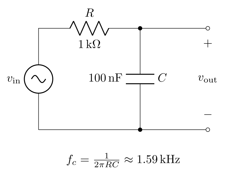
\usepackage{tikz} \usepackage{siunitx} \usepackage[american, RPvoltages]{circuitikz}\begin{circuitikz}
\draw (0,0) to[sV, l=$v_\mathrm{in}$] (0,3)
to[R, l=$R$, a=\qty{1}{\kilo\ohm}] (3,3)
to[C, l=$C$, a=\qty{100}{\nano\farad}, *-*] (3,0) -- (0,0);
\draw (3,3) to[short, -o] (5,3)
(3,0) to[short, -o] (5,0);
% the output voltage between two open terminals
\draw (5,3) to[open, v^=$v_\mathrm{out}$] (5,0);
\node at (2.5,-0.9) {$f_c = \frac{1}{2\pi RC} \approx \qty{1.59}{\kilo\hertz}$};
\end{circuitikz}Full document
\documentclass[border=4pt]{standalone}
\usepackage{tikz}
\usepackage{siunitx}
\usepackage[american, RPvoltages]{circuitikz}
\begin{document}
\begin{circuitikz}
  \draw (0,0) to[sV, l=$v_\mathrm{in}$] (0,3)
        to[R, l=$R$, a=\qty{1}{\kilo\ohm}] (3,3)
        to[C, l=$C$, a=\qty{100}{\nano\farad}, *-*] (3,0) -- (0,0);
  \draw (3,3) to[short, -o] (5,3)
        (3,0) to[short, -o] (5,0);
  % the output voltage between two open terminals
  \draw (5,3) to[open, v^=$v_\mathrm{out}$] (5,0);
  \node at (2.5,-0.9) {$f_c = \frac{1}{2\pi RC} \approx \qty{1.59}{\kilo\hertz}$};
\end{circuitikz}
\end{document}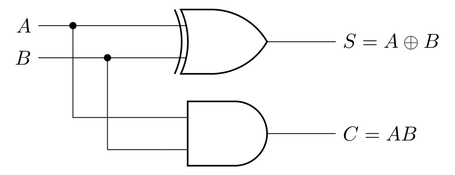
\usepackage{tikz} \usepackage{circuitikz}\begin{circuitikz}
\ctikzset{logic ports=ieee}
% anchor=in 1 keeps the gates aligned on their first input
\draw (0,0) node[xor port, anchor=in 1] (X) {}
(0,-1.6) node[and port, anchor=in 1] (Y) {};
\draw (X.in 1) -- ++(-2.2,0) node[left] {$A$}
(X.in 2) -- ++(-2.2,0) node[left] {$B$};
\draw (X.in 1) ++(-1.6,0) node[circ] {} |- (Y.in 1)
(X.in 2) ++(-1,0) node[circ] {} |- (Y.in 2);
\draw (X.out) -- ++(0.8,0) node[right] {$S = A \oplus B$}
(Y.out) -- ++(0.8,0) node[right] {$C = AB$};
\end{circuitikz}Full document
\documentclass[border=4pt]{standalone}
\usepackage{tikz}
\usepackage{circuitikz}
\begin{document}
\begin{circuitikz}
  \ctikzset{logic ports=ieee}
  % anchor=in 1 keeps the gates aligned on their first input
  \draw (0,0) node[xor port, anchor=in 1] (X) {}
        (0,-1.6) node[and port, anchor=in 1] (Y) {};
  \draw (X.in 1) -- ++(-2.2,0) node[left] {$A$}
        (X.in 2) -- ++(-2.2,0) node[left] {$B$};
  \draw (X.in 1) ++(-1.6,0) node[circ] {} |- (Y.in 1)
        (X.in 2) ++(-1,0) node[circ] {} |- (Y.in 2);
  \draw (X.out) -- ++(0.8,0) node[right] {$S = A \oplus B$}
        (Y.out) -- ++(0.8,0) node[right] {$C = AB$};
\end{circuitikz}
\end{document}The CircuiTikZ manual
The official manual is the CircuiTikZ manual on CTAN (PDF, about 300 pages, version 1.8.7); texdoc circuitikz opens the copy installed with your TeX distribution. The parts you will use most:
- §1.12 package options, §2 four tutorials (current shunt, non-inverting amplifier, transistor amplifier, logic circuit);
- §4 the complete list of components with every name, alias and anchor;
- §5 labels, voltages, currents and flows; §6.1 poles; §8 FAQ (gaps in wires, dashed wires, externalization, scaling).
Check the version you have with \pgfcircversion. If an update changes an old circuit, the package can roll back: \usepackage{circuitikz}[=v1.7.2] (eleven old versions, from 0.4 to 1.7.2, are kept). Questions go to the circuitikz tag on TeX Stack Exchange, bugs to the project’s GitHub issues.
CircuiTikZ designer and other editors
- CircuiTikZ Designer, from the Institute for Electronics Engineering at FAU Erlangen-Nürnberg, is a free browser application for drawing circuits with most CircuiTikZ components and right-angled wires; it exports CircuiTikZ code. The manual also mentions Heaviside, a desktop editor from the University of Colorado Colorado Springs that generates CircuiTikZ code with a live preview.
- The LabCanvas TikZ editor works from code: paste a
circuitikzenvironment, with the package already loaded, and it is typeset with TeX Live as you type, the same renderer as the pictures on this page. Code exported from a designer can be finished there by hand. - “TikZ circuit” can also mean TikZ’s own circuit libraries (
circuits.ee.IEC,circuits.logic.USand others, §49 of the PGF manual), a separate system with its own syntax. They define some of the same style names as CircuiTikZ, so to load both use thecompatibilitypackage option, after which CircuiTikZ’s path components take an asterisk:to[*R].
Common errors and how to fix them
| LaTeX says (or you see) | Cause and fix |
|---|---|
| LaTeX Error: Environment circuitikz undefined. | Add \usepackage{circuitikz} to the preamble. |
| Package pgfkeys Error: I do not know the key '/tikz/R', to which you passed '$R_1$', and I am going to ignore it. | CircuiTikZ is not loaded (only TikZ is), or the component name is misspelt; names are case-sensitive (R, not r). |
| Extra }, or forgotten $. | A label contains = or ,, as in to[R=$R_1=10\,\Omega$]. Brace it: to[R={$R_1=10\,\Omega$}]. |
| Undefined control sequence (in a label such as l=2<\kilo\ohm>) | The <…> unit syntax needs the siunitx package option. Better: \usepackage{siunitx} and l=\qty{2}{\kilo\ohm}. |
| Gaps in the wires at a named point | The point was named with an empty node, which has a size. Name points with coordinate (A) instead (manual FAQ 8.1). |
| A dashed or coloured wire makes the whole path dashed or coloured | Colour and dash options apply to an entire path. Draw that wire as a separate \draw, or as an edge[dashed] (manual FAQ 8.2). |
| ! Emergency stop. (with \tikzexternalize) | The externalization library expects pictures to end with \end{tikzpicture}: use tikzpicture instead of the circuitikz environment (manual FAQ 8.3). |
| The circuit is garbled after yscale=-1, rotate=… or unequal xscale/yscale | Global negative scaling, rotation and non-uniform scaling are not supported (manual §1.8). Flip single components with mirror or invert, and scale the whole circuit with scale=…, transform shape or \scalebox. |
Frequently asked questions
How do I draw a circuit in LaTeX?
Use CircuiTikZ: \usepackage{circuitikz}, then \begin{circuitikz} \draw (0,0) to[V] (0,2) to[R=$R$] (2,2) to[C=$C$] (2,0) -- (0,0); \end{circuitikz}. Each to[…] puts a component on the segment between two points.
How do I draw a voltage source in CircuiTikZ?
to[V] draws the source of the current style (European by default; load [american] for the +/− symbol), vsourceAM always draws the American one, battery1 a battery cell and sV an AC source. The + follows the drawing direction and the voltage option; with RPvoltages it is at the end of the path, and invert turns it round.
How do I draw a switch in CircuiTikZ?
On a path: to[nos] (normally open), to[ncs] (normally closed), to[spst] (closing switch with arrow), to[nopb] (push button), to[cosw] (cute open switch). A changeover switch is a node: node[spdt] (S) {} with anchors S.in, S.out 1, S.out 2.
Where is the CircuiTikZ manual?
On CTAN as a PDF (circuitikzmanual.pdf, linked below), and on your computer with texdoc circuitikz. Chapter 4 lists every component name and anchor.
How do I make the components smaller or the circuit bigger?
\ctikzset{bipoles/length=.8cm} changes the size of all two-terminal components (default 1.4 cm) without changing your coordinates. To scale everything, use \begin{circuitikz}[scale=.8, transform shape], or \scalebox for large factors.
Is there a CircuiTikZ designer or GUI?
Yes: CircuiTikZ Designer (circuit2tikz.tf.fau.de/designer) is a free browser tool that exports CircuiTikZ code. To edit the code and see the result immediately, use the LabCanvas TikZ editor, which typesets circuitikz with TeX Live.
References
- CircuiTikZ package on CTAN (v1.8.7, 2026-09-12)ctan.org
- CircuiTikZ manual (PDF on CTAN)mirrors.ctan.org
- CircuiTikZ manual, §1.12 Package optionsmirrors.ctan.org
- CircuiTikZ manual, §2 Tutorialsmirrors.ctan.org
- CircuiTikZ manual, §3.1 Path-style componentsmirrors.ctan.org
- CircuiTikZ manual, §4.1 Grounds and supply voltagesmirrors.ctan.org
- CircuiTikZ manual, §4.5 Sources and generatorsmirrors.ctan.org
- CircuiTikZ manual, §4.15 Transistorsmirrors.ctan.org
- CircuiTikZ manual, §4.20 Amplifiersmirrors.ctan.org
- CircuiTikZ manual, §4.21 Switches, buttons and jumpersmirrors.ctan.org
- CircuiTikZ manual, §4.22 Logic gatesmirrors.ctan.org
- CircuiTikZ manual, §5 Labels, voltages and currentsmirrors.ctan.org
- CircuiTikZ manual, §6.1 Nodes (poles)mirrors.ctan.org
- CircuiTikZ manual, §8 FAQmirrors.ctan.org
- PGF/TikZ manual, §14.13 The To Path Operationtikz.dev
- PGF/TikZ manual, §13.3.1 Intersections of Perpendicular Lines (-| and |-)tikz.dev
- PGF/TikZ manual, §49 Circuit Librariestikz.dev
- CircuiTikZ Designer (FAU)circuit2tikz.tf.fau.de
The facts on this page were checked against these sources, and every picture is the code with it typeset with TeX Live 2026. Code on this page: CC0 1.0, copy it freely.
Try the code in your browserEvery snippet on this page opens in the free TikZ editor: it is typeset with TeX Live as you type, with errors pointed at their line.
Open the TikZ editor