Converting TikZ to SVG, EPS, PNG and PDF, and plots into TikZ
Quick answer
standalone class: \documentclass[border=2pt]{standalone} gives a PDF cropped to the figure, which is the vector original for everything else. Convert that PDF with standard tools: pdftocairo -svg figure.pdf figure.svg for SVG, pdftocairo -png -r 600 -transp -singlefile figure.pdf figure for a 600 dpi PNG, and pdftops -eps figure.pdf figure.eps for EPS. To export every picture of a long document automatically, use TikZ’s external library, which needs -shell-escape. In the other direction, plots from matplotlib or MATLAB become pgfplots code with matplot2tikz (the maintained successor of tikzplotlib) or matlab2tikz.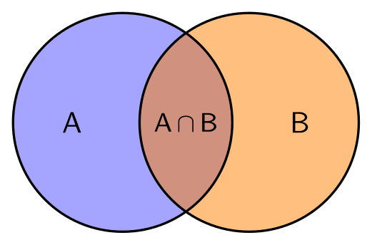
\usepackage{tikz}\begin{tikzpicture}[every node/.style={font=\sffamily}]
% transparent fills: converting to SVG or PNG keeps them, converting to EPS (PostScript) does not
\fill[blue!70, fill opacity=0.5] (0,0) circle [radius=1.3];
\fill[orange, fill opacity=0.5] (1.5,0) circle [radius=1.3];
\draw[thick] (0,0) circle [radius=1.3] (1.5,0) circle [radius=1.3];
\node at (-0.6,0) {A};
\node at (2.1,0) {B};
\node[font=\sffamily\small] at (0.75,0) {A\,$\cap$\,B};
\end{tikzpicture}Full document
\documentclass[border=4pt]{standalone}
\usepackage{tikz}
\begin{document}
\begin{tikzpicture}[every node/.style={font=\sffamily}]
  % transparent fills: converting to SVG or PNG keeps them, converting to EPS (PostScript) does not
  \fill[blue!70, fill opacity=0.5] (0,0) circle [radius=1.3];
  \fill[orange, fill opacity=0.5] (1.5,0) circle [radius=1.3];
  \draw[thick] (0,0) circle [radius=1.3] (1.5,0) circle [radius=1.3];
  \node at (-0.6,0) {A};
  \node at (2.1,0) {B};
  \node[font=\sffamily\small] at (0.75,0) {A\,$\cap$\,B};
\end{tikzpicture}
\end{document}Contents
Step 1: compile the figure on its own (standalone class)
Put the picture in a document of its own with the standalone class. It makes the page exactly as large as the content (it crops by default), plus the margin you give with border:
\documentclass[border=2pt]{standalone}
\usepackage{tikz}
\usetikzlibrary{arrows.meta}   % the libraries your figure uses
\begin{document}
\begin{tikzpicture}
  …
\end{tikzpicture}
\end{document}
pdflatex figure.tex (or LuaLaTeX, XeLaTeX) then writes figure.pdf: a vector file with embedded fonts that LaTeX includes with \includegraphics{figure} and that the converters below turn into anything else. With \documentclass[tikz]{standalone}, every tikzpicture in the file becomes a page of its own, so one file can hold all the figures of a paper. Every snippet on these pages is compiled this way, with border=4pt.
Step 2: convert the PDF to SVG, PNG or EPS
| Target | Command | Notes |
|---|---|---|
| SVG | pdftocairo -svg figure.pdf figure.svg | poppler; text becomes outlined paths, so it looks right everywhere but is not editable as text |
| SVG with real text | \usepackage[dvisvgm]{tikz}, then latex figure and dvisvgm --font-format=woff2 figure | the DVI route of the PGF manual (§10.2.4); --no-fonts writes paths instead; lualatex --output-format=dvi also works |
SVG, converted from figure.pdf | dvisvgm --pdf figure.pdf | needs Ghostscript older than 10.01.0 or the mutool program of MuPDF |
| PNG | pdftocairo -png -r 600 -transp -singlefile figure.pdf figure | writes figure.png at 600 dpi with a transparent background; without -singlefile the page number is added to the name |
| PNG | gs -sDEVICE=png16malpha -r600 -o figure.png figure.pdf | Ghostscript; -o also sets -dBATCH -dNOPAUSE |
| EPS | pdftops -eps figure.pdf figure.eps | poppler, the conversion the TikZ manual suggests; one page per EPS (-f 2 -l 2 picks page 2) |
| EPS | gs -sDEVICE=eps2write -o figure.eps figure.pdf | Ghostscript |
pdftocairo and pdftops are part of poppler (the poppler-utils package on Linux, poppler in Homebrew on macOS); dvisvgm comes with TeX Live, and Windows builds are on its website; Ghostscript is a separate install. For a PNG, the pixel size is the figure size in points ÷ 72 × dpi, so a figure 8.5 cm (241 pt) wide is 2008 pixels wide at 600 dpi.
What each format keeps: transparency, text and size
- PDF, the file LaTeX writes, holds the drawing exactly: lines and text stay sharp at any size, with the fonts embedded, transparency (
opacity,fill opacity) and shadings. It is the best file for a journal that accepts PDF figures. - SVG keeps vectors and transparency. Whether text stays text depends on the converter: pdftocairo outlines it, dvisvgm can embed WOFF fonts that browsers understand but many drawing programs do not.
- EPS is PostScript, which has no transparency. Ghostscript’s documentation says that a page with PDF transparency is then rendered as a whole to a bitmap and wrapped in the EPS, so the result is no longer vector. If a journal requires EPS, avoid opacity in the figure, or ask whether it accepts PDF.
- PNG is pixels: choose the dpi for the final printed size (300 for photos and slides, 600 or more for line art) and never enlarge it later.
The Venn diagram at the top uses fill opacity: converting it to SVG or PNG keeps the transparency, converting it to EPS does not.
Tight cropping: empty space around curves, and a fixed size
The cropped size is TikZ’s bounding box, and for curves TikZ counts the Bézier control points, which can lie far outside the curve. The exported image then has empty space above or below. Load \usetikzlibrary{bbox} (from the tikz-bbox package, in TeX Live) and add bezier bounding box to the picture to compute the real extent of the curves.
For figures that must have an exact size, for example panels that will be placed side by side, fix the bounding box yourself: \useasboundingbox (0,0) rectangle (8.5,2.5); makes the picture 8.5 cm × 2.5 cm whatever is drawn, and anything outside is cut off when the PDF is cropped. overlay on a path or node does the opposite: it is drawn but not counted for the size.
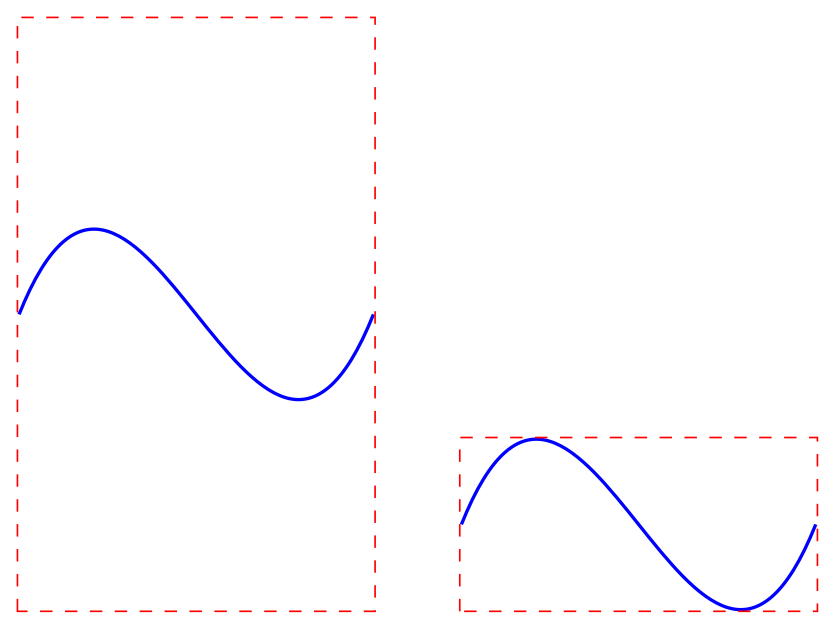
\usepackage{tikz} \usetikzlibrary{bbox}% left: TikZ counts the control points, so the cropped image gets empty space
\begin{tikzpicture}
\draw[thick, blue] (0,0) .. controls (1,2.5) and (2,-2.5) .. (3,0);
\draw[red, dashed] (current bounding box.south west) rectangle (current bounding box.north east);
\end{tikzpicture}\qquad
% right: the bbox library computes the curve's real extent
\begin{tikzpicture}[bezier bounding box]
\draw[thick, blue] (0,0) .. controls (1,2.5) and (2,-2.5) .. (3,0);
\draw[red, dashed] (current bounding box.south west) rectangle (current bounding box.north east);
\end{tikzpicture}Full document
\documentclass[border=4pt]{standalone}
\usepackage{tikz}
\usetikzlibrary{bbox}
\begin{document}
% left: TikZ counts the control points, so the cropped image gets empty space
\begin{tikzpicture}
  \draw[thick, blue] (0,0) .. controls (1,2.5) and (2,-2.5) .. (3,0);
  \draw[red, dashed] (current bounding box.south west) rectangle (current bounding box.north east);
\end{tikzpicture}\qquad
% right: the bbox library computes the curve's real extent
\begin{tikzpicture}[bezier bounding box]
  \draw[thick, blue] (0,0) .. controls (1,2.5) and (2,-2.5) .. (3,0);
  \draw[red, dashed] (current bounding box.south west) rectangle (current bounding box.north east);
\end{tikzpicture}
\end{document}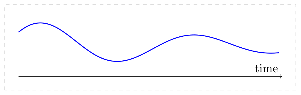
\usepackage{tikz}\begin{tikzpicture}
% the picture is exactly 8.5 cm x 2.5 cm, whatever is drawn inside
\useasboundingbox (0,0) rectangle (8.5,2.5);
\draw[gray, dashed] (0,0) rectangle (8.5,2.5); % only to show the frame
\draw[->] (0.4,0.4) -- (8.1,0.4) node[above left] {time};
\draw[blue, thick, smooth, domain=0.4:8, samples=60, variable=\t]
plot ({\t}, {1.3 + 0.8*sin(deg(1.4*\t))*exp(-\t/6)});
\end{tikzpicture}Full document
\documentclass[border=4pt]{standalone}
\usepackage{tikz}
\begin{document}
\begin{tikzpicture}
  % the picture is exactly 8.5 cm x 2.5 cm, whatever is drawn inside
  \useasboundingbox (0,0) rectangle (8.5,2.5);
  \draw[gray, dashed] (0,0) rectangle (8.5,2.5);   % only to show the frame
  \draw[->] (0.4,0.4) -- (8.1,0.4) node[above left] {time};
  \draw[blue, thick, smooth, domain=0.4:8, samples=60, variable=\t]
    plot ({\t}, {1.3 + 0.8*sin(deg(1.4*\t))*exp(-\t/6)});
\end{tikzpicture}
\end{document}Scaling a figure for export without breaking the text
Draw the figure at its final size where you can. If it has to shrink, know what each method does: scale=0.6 on the picture moves the coordinates closer but keeps nodes and text at their size, so boxes can overlap; adding transform shape scales nodes and text too, so 10 pt text becomes 6 pt; \resizebox{8.5cm}{!}{…} around the picture does the same as the latter. A journal that asks for a minimum font size in figures (often 6–8 pt) checks the printed size, so shrink the drawing, not the text: reduce distances and node sizes, or use pgfplots’ width, which keeps the font size.
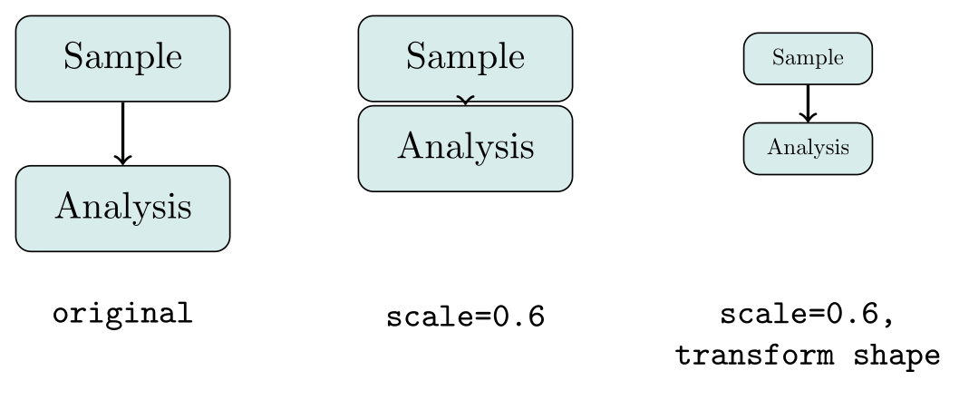
\usepackage{tikz}\begin{tikzpicture}[box/.style={draw, rounded corners, fill=teal!15, minimum width=2cm, minimum height=0.8cm}]
% original size
\node[box] (a) at (0,0) {Sample};
\node[box] (b) at (0,-1.4) {Analysis};
\draw[->, thick] (a) -- (b);
\node[font=\ttfamily\small] at (0,-2.4) {original};
% scale=0.6: coordinates shrink, text and node sizes stay
\begin{scope}[xshift=3.2cm, scale=0.6]
\node[box] (a) at (0,0) {Sample};
\node[box] (b) at (0,-1.4) {Analysis};
\draw[->, thick] (a) -- (b);
\end{scope}
\node[font=\ttfamily\small] at (3.2,-2.4) {scale=0.6};
% transform shape: nodes and text shrink too
\begin{scope}[xshift=6.4cm, scale=0.6, transform shape]
\node[box] (a) at (0,0) {Sample};
\node[box] (b) at (0,-1.4) {Analysis};
\draw[->, thick] (a) -- (b);
\end{scope}
\node[font=\ttfamily\small, align=center] at (6.4,-2.6) {scale=0.6,\\transform shape};
\end{tikzpicture}Full document
\documentclass[border=4pt]{standalone}
\usepackage{tikz}
\begin{document}
\begin{tikzpicture}[box/.style={draw, rounded corners, fill=teal!15, minimum width=2cm, minimum height=0.8cm}]
  % original size
  \node[box] (a) at (0,0) {Sample};
  \node[box] (b) at (0,-1.4) {Analysis};
  \draw[->, thick] (a) -- (b);
  \node[font=\ttfamily\small] at (0,-2.4) {original};
  % scale=0.6: coordinates shrink, text and node sizes stay
  \begin{scope}[xshift=3.2cm, scale=0.6]
    \node[box] (a) at (0,0) {Sample};
    \node[box] (b) at (0,-1.4) {Analysis};
    \draw[->, thick] (a) -- (b);
  \end{scope}
  \node[font=\ttfamily\small] at (3.2,-2.4) {scale=0.6};
  % transform shape: nodes and text shrink too
  \begin{scope}[xshift=6.4cm, scale=0.6, transform shape]
    \node[box] (a) at (0,0) {Sample};
    \node[box] (b) at (0,-1.4) {Analysis};
    \draw[->, thick] (a) -- (b);
  \end{scope}
  \node[font=\ttfamily\small, align=center] at (6.4,-2.6) {scale=0.6,\\transform shape};
\end{tikzpicture}
\end{document}Fonts in exported figures
The exported figure uses the fonts of the standalone document, Computer Modern unless you load another. To match a document in Times, load the same font package in the figure (for example newtxtext and newtxmath). Many journals ask for a sans-serif font such as Helvetica or Arial in figures: \usepackage[scaled]{helvet} with font=\sffamily changes the text, but numbers in pgfplots tick labels are typeset in math mode and stay serif until you also switch math to sans-serif, for example with the sansmath package and \sansmath, as below. With LuaLaTeX or XeLaTeX, fontspec can load any installed font.
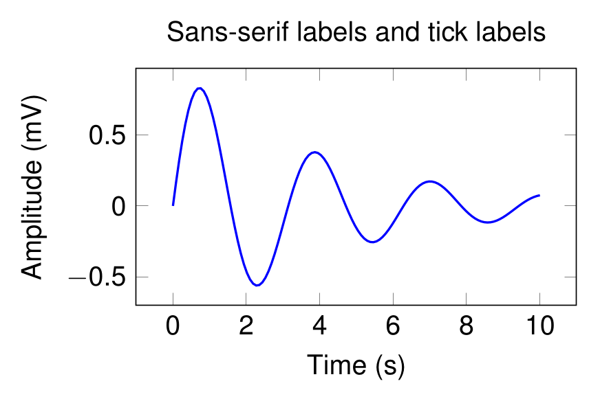
\usepackage{tikz} \usepackage{pgfplots} \pgfplotsset{compat=1.18} \usepackage[T1]{fontenc} \usepackage[scaled]{helvet} \usepackage{sansmath}% Helvetica for text, and \sansmath because tick labels are typeset in math mode
\begin{tikzpicture}[font=\sffamily\sansmath]
\begin{axis}[
width=7cm, height=4.5cm,
xlabel={Time (s)}, ylabel={Amplitude (mV)},
title={Sans-serif labels and tick labels},
]
\addplot[blue, thick, domain=0:10, samples=120] {exp(-x/4)*sin(deg(2*x))};
\end{axis}
\end{tikzpicture}Full document
\documentclass[border=4pt]{standalone}
\usepackage{tikz}
\usepackage{pgfplots}
\pgfplotsset{compat=1.18}
\usepackage[T1]{fontenc}
\usepackage[scaled]{helvet}
\usepackage{sansmath}
\begin{document}
% Helvetica for text, and \sansmath because tick labels are typeset in math mode
\begin{tikzpicture}[font=\sffamily\sansmath]
  \begin{axis}[
      width=7cm, height=4.5cm,
      xlabel={Time (s)}, ylabel={Amplitude (mV)},
      title={Sans-serif labels and tick labels},
    ]
    \addplot[blue, thick, domain=0:10, samples=120] {exp(-x/4)*sin(deg(2*x))};
  \end{axis}
\end{tikzpicture}
\end{document}The external library: export every picture of a document
In a document with many figures, TikZ can write each picture to its own PDF and reuse it on later runs, which saves compilation time and leaves you with a file per figure:
\usetikzlibrary{external}
\tikzexternalize[prefix=figures/]   % in the preamble; create the folder figures/

\tikzsetnextfilename{workflow}      % optional: figures/workflow.pdf instead of figures/main-figure0.pdf
\begin{tikzpicture} … \end{tikzpicture}
By default (mode=convert with system call) the library calls LaTeX itself for each picture, which requires shell escape: pdflatex -shell-escape main.tex (MiKTeX: \tikzexternalize[shell escape=-enable-write18]). Without it, LaTeX stops with the “did NOT result in a usable output file” error below. mode=list and make needs no shell escape: LaTeX writes main.makefile, you run make -f main.makefile, and the next LaTeX run includes the files. A picture is regenerated when its code changes. For EPS files, the manual suggests adding pdftops -eps to the system call. On Overleaf, externalizing needs a little setup; see TikZ on Overleaf.
What the LabCanvas TikZ editor exports
The LabCanvas TikZ editor typesets your code with TeX Live 2026 on LabCanvas servers, the same renderer that made the pictures on this page. It gives you a transparent PNG at 300 or 600 dpi, with the dpi written into the file so that Word and PowerPoint place it at its real size, or it opens the figure in the LabCanvas editor as editable vector shapes (text as outlines) to combine with plots and images there. Those shapes stay inside LabCanvas: there is no SVG, EPS or PDF download. For those formats, compile the code locally and use the commands above.
The editor runs without shell escape, so the external library, standalone’s convert option and gnuplot-based plots do not work there, and each render has 25 seconds; a document with several pages shows its first page.
Plots into TikZ: tikzplotlib, matplot2tikz, matlab2tikz, or the data
| Tool | From | Latest release | Status |
|---|---|---|---|
| tikzplotlib | matplotlib | 0.10.1, 31 Jan 2022 | No release since 2022 (the repository is not archived). It imports a function that matplotlib removed in version 3.8 (September 2023), so import tikzplotlib fails with any current matplotlib. |
| matplot2tikz | matplotlib | 0.5.4, 23 Mar 2026 | The maintained fork (“the artist formerly known as tikzplotlib”), same API: pip install matplot2tikz, then matplot2tikz.save("figure.tex"). Python 3.10 or newer. |
| matlab2tikz | MATLAB, Octave | 1.1.0, 20 Oct 2016 | No release since 2016, repository not archived. matlab2tikz('figure.tex'); cleanfigure first removes points outside the axes. |
| matplotlib’s pgf backend | matplotlib | part of matplotlib | plt.savefig("figure.pgf") writes low-level PGF drawing commands for \input, not pgfplots code: exact, but hard to edit. |
The output of a converter is a starting point. The snippet below is matplot2tikz’s unchanged output for a small matplotlib figure: it compiles as is, and copies matplotlib’s colours, limits and legend style; it sets no width, so pgfplots uses its default 240 pt × 207 pt (pass axis_width="8cm" to change that). The colours get generated names such as steelblue31119180, and the data are written inline. Renaming the colours and moving the data into a file is usually the first edit.
Often cleaner: export only the data (np.savetxt, pandas.DataFrame.to_csv, MATLAB’s writematrix or writetable) and plot them with \addplot table, so the plot follows the style of the rest of the document. \pgfplotstableread reads the file once for several plots; computing a column with y expr from such a table needs \usepackage{pgfplotstable}. More on plotting on the pgfplots page.
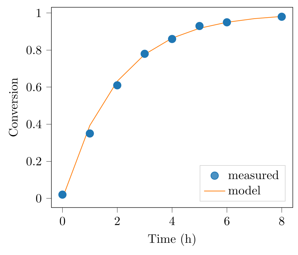
\usepackage{tikz} \usepackage{pgfplots} \pgfplotsset{compat=1.18}% written by matplot2tikz 0.5.4 from a matplotlib 3.11.2 figure (unchanged apart from this line)
\begin{tikzpicture}
\definecolor{darkgray176}{RGB}{176,176,176}
\definecolor{darkorange25512714}{RGB}{255,127,14}
\definecolor{lightgray204}{RGB}{204,204,204}
\definecolor{steelblue31119180}{RGB}{31,119,180}
\begin{axis}[
legend cell align={left},
legend style={
fill opacity=0.8,
draw opacity=1,
text opacity=1,
at={(0.97,0.03)},
anchor=south east,
draw=lightgray204
},
tick align=outside,
tick pos=left,
x grid style={darkgray176},
xlabel={Time (h)},
xmin=-0.4, xmax=8.4,
xtick style={color=black},
y grid style={darkgray176},
ylabel={Conversion},
ymin=-0.0490842180555633, ymax=1.03076857916683,
ytick style={color=black}
]
\addplot [semithick, steelblue31119180, mark=*, mark size=3, mark options={solid}, only marks]
table {%
0 0.02
1 0.35
2 0.61
3 0.78
4 0.86
5 0.93
6 0.95
8 0.98
};
\addlegendentry{measured}
\addplot [semithick, darkorange25512714]
table {%
0 0
1 0.393469340287367
2 0.632120558828558
3 0.77686983985157
4 0.864664716763387
5 0.917915001376101
6 0.950212931632136
7 0.969802616577682
8 0.981684361111266
};
\addlegendentry{model}
\end{axis}
\end{tikzpicture}Full document
\documentclass[border=4pt]{standalone}
\usepackage{tikz}
\usepackage{pgfplots}
\pgfplotsset{compat=1.18}
\begin{document}
% written by matplot2tikz 0.5.4 from a matplotlib 3.11.2 figure (unchanged apart from this line)
\begin{tikzpicture}

\definecolor{darkgray176}{RGB}{176,176,176}
\definecolor{darkorange25512714}{RGB}{255,127,14}
\definecolor{lightgray204}{RGB}{204,204,204}
\definecolor{steelblue31119180}{RGB}{31,119,180}

\begin{axis}[
legend cell align={left},
legend style={
  fill opacity=0.8,
  draw opacity=1,
  text opacity=1,
  at={(0.97,0.03)},
  anchor=south east,
  draw=lightgray204
},
tick align=outside,
tick pos=left,
x grid style={darkgray176},
xlabel={Time (h)},
xmin=-0.4, xmax=8.4,
xtick style={color=black},
y grid style={darkgray176},
ylabel={Conversion},
ymin=-0.0490842180555633, ymax=1.03076857916683,
ytick style={color=black}
]
\addplot [semithick, steelblue31119180, mark=*, mark size=3, mark options={solid}, only marks]
table {%
0 0.02
1 0.35
2 0.61
3 0.78
4 0.86
5 0.93
6 0.95
8 0.98
};
\addlegendentry{measured}
\addplot [semithick, darkorange25512714]
table {%
0 0
1 0.393469340287367
2 0.632120558828558
3 0.77686983985157
4 0.864664716763387
5 0.917915001376101
6 0.950212931632136
7 0.969802616577682
8 0.981684361111266
};
\addlegendentry{model}
\end{axis}

\end{tikzpicture}
\end{document}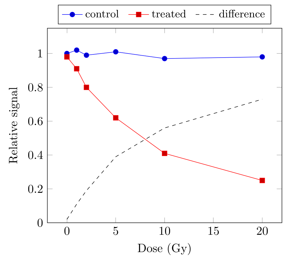
\usepackage{tikz} \usepackage{pgfplots} \pgfplotsset{compat=1.18} \usepackage{pgfplotstable}\begin{tikzpicture}
% a CSV file saved by Python, MATLAB, R or a spreadsheet, read once into \results;
% in a document: \pgfplotstableread[col sep=comma]{results.csv}\results
\pgfplotstableread[col sep=comma]{
dose,control,treated
0,1.00,0.98
1,1.02,0.91
2,0.99,0.80
5,1.01,0.62
10,0.97,0.41
20,0.98,0.25
}\results
\begin{axis}[xlabel={Dose (Gy)}, ylabel={Relative signal}, ymin=0, ymax=1.15,
legend style={at={(0.5,1.02)}, anchor=south, legend columns=-1, font=\small,
/tikz/every even column/.append style={column sep=0.2cm}}]
\addplot table[x=dose, y=control] {\results};
\addlegendentry{control}
\addplot table[x=dose, y=treated] {\results};
\addlegendentry{treated}
% a column computed from two others
\addplot[black, dashed] table[x=dose, y expr=\thisrow{control}-\thisrow{treated}] {\results};
\addlegendentry{difference}
\end{axis}
\end{tikzpicture}Full document
\documentclass[border=4pt]{standalone}
\usepackage{tikz}
\usepackage{pgfplots}
\pgfplotsset{compat=1.18}
\usepackage{pgfplotstable}
\begin{document}
\begin{tikzpicture}
  % a CSV file saved by Python, MATLAB, R or a spreadsheet, read once into \results;
  % in a document: \pgfplotstableread[col sep=comma]{results.csv}\results
  \pgfplotstableread[col sep=comma]{
    dose,control,treated
    0,1.00,0.98
    1,1.02,0.91
    2,0.99,0.80
    5,1.01,0.62
    10,0.97,0.41
    20,0.98,0.25
  }\results
  \begin{axis}[xlabel={Dose (Gy)}, ylabel={Relative signal}, ymin=0, ymax=1.15,
               legend style={at={(0.5,1.02)}, anchor=south, legend columns=-1, font=\small,
                             /tikz/every even column/.append style={column sep=0.2cm}}]
    \addplot table[x=dose, y=control] {\results};
    \addlegendentry{control}
    \addplot table[x=dose, y=treated] {\results};
    \addlegendentry{treated}
    % a column computed from two others
    \addplot[black, dashed] table[x=dose, y expr=\thisrow{control}-\thisrow{treated}] {\results};
    \addlegendentry{difference}
  \end{axis}
\end{tikzpicture}
\end{document}TikZ download, tikz.sty and the GitHub repository
TikZ is not a separate download. It is part of the pgf package (version 3.1.12 of August 2026), which every TeX distribution includes: TeX Live installs it with the standard schemes (or tlmgr install pgf), MiKTeX installs it automatically the first time a document asks for it, and Overleaf has it already. kpsewhich tikz.sty shows where it is installed, and \pgfversion typeset in a document prints the version.
Downloading tikz.sty by itself does not work: the file only loads pgf, pgffor and tikz.code.tex, which in turn load hundreds of other files of the bundle. For a manual installation, take the whole package from CTAN (the TDS zip unpacks into a local texmf tree). The source code, issue tracker and releases are on GitHub at pgf-tikz/pgf; the manual is on tikz.dev and in your installation as texdoc pgf.
Common errors and how to fix them
| LaTeX says (or you see) | Cause and fix |
|---|---|
| Package tikz Error: Sorry, the system call 'pdflatex -halt-on-error -interaction=batchmode -jobname "main-figure0" "\def\tikzexternalrealjob{main}\input{main}"' did NOT result in a usable output file 'main-figure0' (expected one of .pdf:.jpg:.jpeg:.png:). Please verify that you have enabled system calls. For pdflatex, this is 'pdflatex -shell-escape'. … | The external library could not run LaTeX for the picture because shell escape is off. Compile with pdflatex -shell-escape (MiKTeX: -enable-write18), or use \tikzexternalize[mode=list and make] and run make -f main.makefile. |
| EPS files can only contain one page. | pdftocairo -eps was given a file with several pages (for example from \documentclass[tikz]{standalone}). Pick one page with -f 2 -l 2, or convert each page separately. |
| ImportError: cannot import name 'common_texification' from 'matplotlib.backends.backend_pgf' | tikzplotlib 0.10.1 does not work with matplotlib 3.8 or newer, which removed that function. Install the maintained fork instead: pip install matplot2tikz, and call matplot2tikz.save("figure.tex"). |
| LaTeX Error: File `tikz.sty' not found. | The pgf package is missing from this TeX installation: tlmgr install pgf (TeX Live), let MiKTeX install it on demand, or install a full TeX distribution. Copying tikz.sty alone does not help. |
| Package pgfplotstable Error: Please load \usepackage{pgfplotstable} before using \pgfplotstablecreatecol. | y expr (or another computed column) was used on a table read with \pgfplotstableread. Add \usepackage{pgfplotstable} to the preamble. |
| The exported image has empty space above or below a curve (no error) | TikZ counts the Bézier control points in the bounding box. Load \usetikzlibrary{bbox} and add bezier bounding box to the picture, or set the size with \useasboundingbox. |
| The EPS file is blurry or very large (no error) | The figure uses transparency, which PostScript cannot represent, so the converter rendered it as a bitmap. Remove opacity from the figure or submit PDF instead of EPS. |
| Text in the SVG cannot be edited (no error) | pdftocairo writes text as outlined paths. For text elements, go through DVI: \usepackage[dvisvgm]{tikz}, latex, then dvisvgm with --font-format=woff2. |
Frequently asked questions
How do I convert TikZ to SVG?
Compile the picture with \documentclass[border=2pt]{standalone} to get a cropped PDF, then run pdftocairo -svg figure.pdf figure.svg (text becomes paths). For SVG with real text, load \usepackage[dvisvgm]{tikz}, compile with latex and convert the DVI with dvisvgm. LabCanvas does not offer an SVG download.
How do I export a TikZ figure as EPS?
Make a cropped PDF with the standalone class, then pdftops -eps figure.pdf figure.eps, or gs -sDEVICE=eps2write -o figure.eps figure.pdf. There is no transparency in EPS: figures with opacity are turned into bitmaps, so remove the opacity, or ask whether the journal accepts the PDF.
Where do I download TikZ or tikz.sty?
Nowhere separately: TikZ is part of the pgf package that comes with TeX Live, MiKTeX and Overleaf. If LaTeX cannot find tikz.sty, install pgf with your distribution’s package manager (tlmgr install pgf in TeX Live). The source is on GitHub at pgf-tikz/pgf and on CTAN.
Is tikzplotlib still maintained?
No release has appeared since 0.10.1 in January 2022, and it fails to import with matplotlib 3.8 and newer. matplot2tikz is the maintained fork with the same interface (pip install matplot2tikz; matplot2tikz.save("figure.tex")); version 0.5.4 came out in March 2026.
Does matlab2tikz still work?
It is still available on GitHub and MATLAB File Exchange, but its latest release is 1.1.0 from October 2016, so recent MATLAB graphics features may not convert. Run cleanfigure, then matlab2tikz('figure.tex'), and check the result; exporting the data with writematrix and plotting them with pgfplots is the robust alternative.
Can I get a PNG of TikZ code without installing LaTeX?
Yes: paste the code into the LabCanvas TikZ editor, which typesets it with TeX Live and downloads a transparent PNG at 300 or 600 dpi, or opens it as editable shapes in the LabCanvas editor. Vector downloads (SVG, EPS, PDF) are not offered there.
References
- standalone class on CTAN (v1.5a): cropping, the tikz and convert optionsctan.org
- PGF/TikZ manual, §10.2.4: the dvisvgm driver for SVGtikz.dev
- PGF/TikZ manual, §15.8 Establishing a Bounding Boxtikz.dev
- PGF/TikZ manual, §17.7 Transformations (transform shape)tikz.dev
- PGF/TikZ manual, §52.4 Externalizing Graphicstikz.dev
- PGF/TikZ manual, §52.6: EPS files from the external librarytikz.dev
- pgfplots manual 1.18.3, §7.1: externalizing pgfplots figures (p. 538)mirrors.ctan.org
- pgfplots manual, §4.3.2 Reading Coordinates From Tablestikz.dev
- pgfplotstable manual (PDF on CTAN)mirrors.ctan.org
- tikz-bbox on CTAN (v0.1): the bbox library and bezier bounding boxctan.org
- pdftocairo manual page (poppler-utils)manpages.debian.org
- pdftops manual page (poppler-utils)manpages.debian.org
- dvisvgm manual page (current version 3.6.1)dvisvgm.de
- Ghostscript documentation: the -o optionghostscript.readthedocs.io
- Ghostscript documentation: high-level devices (eps2write, transparency)ghostscript.readthedocs.io
- matplot2tikz on PyPI (0.5.4, 2026-03-23)pypi.org
- tikzplotlib on PyPI (0.10.1, 2022-01-31)pypi.org
- matplotlib 3.8.0 API changes (backend_pgf.common_texification removed)matplotlib.org
- matplotlib: text rendering with the pgf backendmatplotlib.org
- matlab2tikz on MATLAB File Exchange (v1.1.0)mathworks.com
- pgf package on CTAN (v3.1.12)ctan.org
- sansmath package on CTANctan.org
The facts on this page were checked against these sources, and every picture is the code with it typeset with TeX Live 2026. Code on this page: CC0 1.0, copy it freely.
Try the code in your browserEvery snippet on this page opens in the free TikZ editor: it is typeset with TeX Live as you type, with errors pointed at their line.
Open the TikZ editor