TikZ plots with pgfplots: functions, data, scatter, bars and 3D
Quick answer
pgfplots, the plotting package built on TikZ: load \usepackage{pgfplots} and \pgfplotsset{compat=1.18}, put an axis environment inside a tikzpicture, and add one \addplot per data series. \addplot {x^2}; plots a function, \addplot coordinates {(0,1) (1,3)}; plots points, and \addplot table {…}; reads columns of data. pgfplots chooses the axis limits and ticks; xlabel, legend pos and grid are options of the axis. For a quick curve without axes, plain TikZ has a plot operation.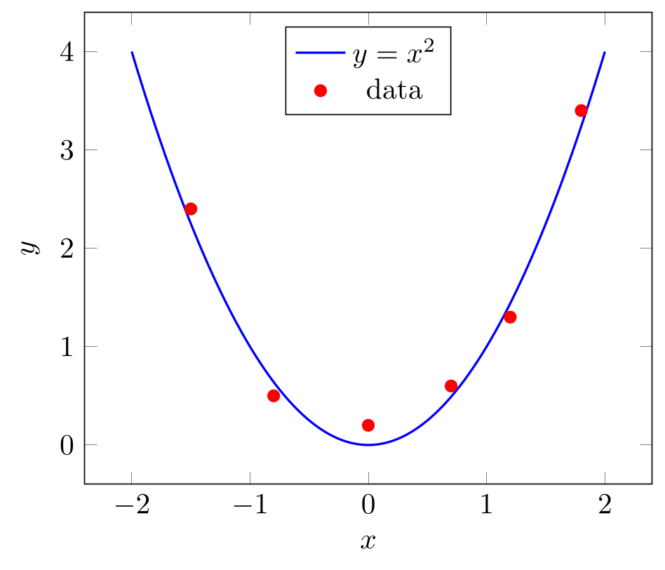
\usepackage{tikz} \usepackage{pgfplots} \pgfplotsset{compat=1.18}\begin{tikzpicture}
\begin{axis}[
xlabel={$x$}, ylabel={$y$},
legend style={at={(0.5,0.97)}, anchor=north},
]
% a function: \addplot {expression in x}
\addplot[blue, thick, domain=-2:2, samples=100] {x^2};
\addlegendentry{$y = x^2$}
% measured points: \addplot coordinates {(x,y) ...}
\addplot[red, only marks, mark=*] coordinates {
(-1.5,2.4) (-0.8,0.5) (0,0.2) (0.7,0.6) (1.2,1.3) (1.8,3.4)
};
\addlegendentry{data}
\end{axis}
\end{tikzpicture}Full document
\documentclass[border=4pt]{standalone}
\usepackage{tikz}
\usepackage{pgfplots}
\pgfplotsset{compat=1.18}
\begin{document}
\begin{tikzpicture}
  \begin{axis}[
      xlabel={$x$}, ylabel={$y$},
      legend style={at={(0.5,0.97)}, anchor=north},
    ]
    % a function: \addplot {expression in x}
    \addplot[blue, thick, domain=-2:2, samples=100] {x^2};
    \addlegendentry{$y = x^2$}
    % measured points: \addplot coordinates {(x,y) ...}
    \addplot[red, only marks, mark=*] coordinates {
      (-1.5,2.4) (-0.8,0.5) (0,0.2) (0.7,0.6) (1.2,1.3) (1.8,3.4)
    };
    \addlegendentry{data}
  \end{axis}
\end{tikzpicture}
\end{document}Contents
The axis environment and compat=1.18
A pgfplots figure is a tikzpicture with an axis environment inside. axis has linear scales; semilogxaxis, semilogyaxis and loglogaxis make the x axis, the y axis or both logarithmic (the same as xmode=log and ymode=log on axis). Options of the axis apply to the whole plot: limits (xmin, xmax, ymin, ymax), labels (xlabel, ylabel, title), the legend and the size. Options of an \addplot apply to that series only, and every \addplot ends with a semicolon.
Always set \pgfplotsset{compat=1.18} in the preamble. Without it, pgfplots runs in a backwards-compatibility mode that keeps the behaviour of very old versions (axis labels placed as before version 1.3, among other things) and says so in the log. 1.18 is the newest level, also in pgfplots 1.18.3 of August 2026; compat follows changes in behaviour, not the package version. compat=newest also exists, but a fixed number keeps the figure the same when pgfplots is updated.
Without options, each \addplot takes the next style from the cycle list (blue with circles, red with squares, brown with crossed circles…). \addplot[red, thick] replaces that style; \addplot+[thick] keeps it and adds to it.
Plotting a function: \addplot with an expression
\addplot {⟨expression in x⟩}; samples the function at samples points (initially 25) evenly spread over domain (initially −5:5), and joins them with straight lines, so raise samples for curved or fast-changing functions. ^ is the power operator, and exp, ln, sqrt, abs, pi and e are available. The trap: trigonometric functions take degrees, so sin(x) over −5:5 looks like a straight line. Write sin(deg(x)), or give the plot (or the axis) trig format plots=rad.
Give domain to the axis to set it for every plot, or to one \addplot for that plot only; the axis limits follow the plots unless you set xmin/xmax. Tick positions accept expressions too (xtick={0, pi/2, pi}) and xticklabels sets their text. For a function with a pole, such as 1/x or tan, add restrict y to domain=-10:10 so that huge values do not stretch the axis. A parametric curve is \addplot ({cos(deg(x))}, {sin(deg(x))});, with x running over the domain.
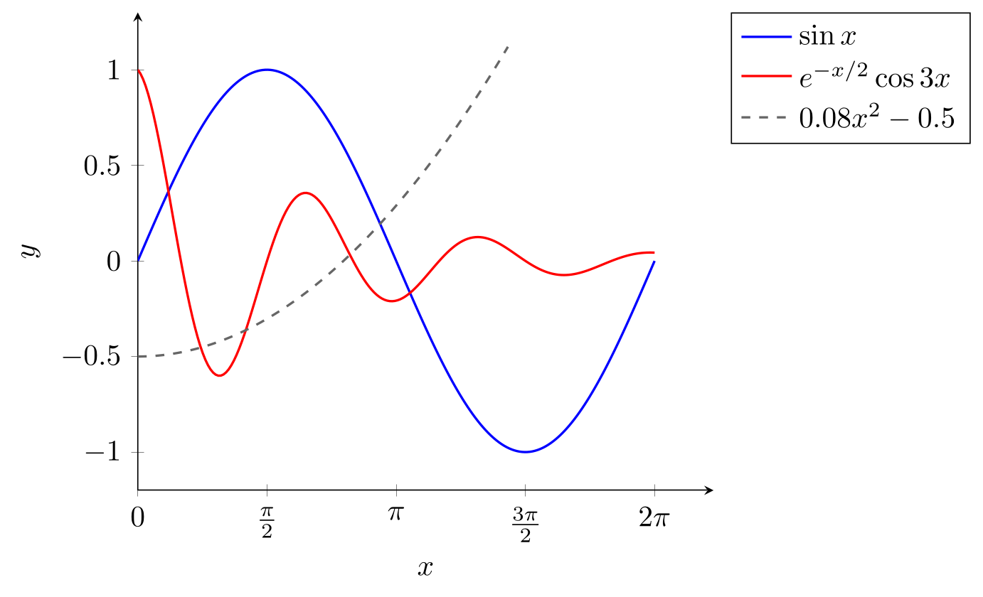
\usepackage{tikz} \usepackage{pgfplots} \pgfplotsset{compat=1.18}\begin{tikzpicture}
\begin{axis}[
domain=0:2*pi, samples=200,
xmin=0, xmax=7, ymin=-1.2, ymax=1.3,
xtick={0, pi/2, pi, 3*pi/2, 2*pi},
xticklabels={$0$, $\frac{\pi}{2}$, $\pi$, $\frac{3\pi}{2}$, $2\pi$},
axis lines=left, xlabel={$x$}, ylabel={$y$},
legend pos=outer north east, legend cell align=left,
]
% trigonometric functions work in degrees: deg() converts x from radians
\addplot[blue, thick] {sin(deg(x))};
\addlegendentry{$\sin x$}
% or switch this plot to radians
\addplot[red, thick, trig format plots=rad] {exp(-x/2)*cos(3*x)};
\addlegendentry{$e^{-x/2}\cos 3x$}
% ^ is the power operator; another domain for one plot only
\addplot[black!60, thick, dashed, domain=0:4.5] {0.08*x^2 - 0.5};
\addlegendentry{$0.08x^2 - 0.5$}
\end{axis}
\end{tikzpicture}Full document
\documentclass[border=4pt]{standalone}
\usepackage{tikz}
\usepackage{pgfplots}
\pgfplotsset{compat=1.18}
\begin{document}
\begin{tikzpicture}
  \begin{axis}[
      domain=0:2*pi, samples=200,
      xmin=0, xmax=7, ymin=-1.2, ymax=1.3,
      xtick={0, pi/2, pi, 3*pi/2, 2*pi},
      xticklabels={$0$, $\frac{\pi}{2}$, $\pi$, $\frac{3\pi}{2}$, $2\pi$},
      axis lines=left, xlabel={$x$}, ylabel={$y$},
      legend pos=outer north east, legend cell align=left,
    ]
    % trigonometric functions work in degrees: deg() converts x from radians
    \addplot[blue, thick] {sin(deg(x))};
    \addlegendentry{$\sin x$}
    % or switch this plot to radians
    \addplot[red, thick, trig format plots=rad] {exp(-x/2)*cos(3*x)};
    \addlegendentry{$e^{-x/2}\cos 3x$}
    % ^ is the power operator; another domain for one plot only
    \addplot[black!60, thick, dashed, domain=0:4.5] {0.08*x^2 - 0.5};
    \addlegendentry{$0.08x^2 - 0.5$}
  \end{axis}
\end{tikzpicture}
\end{document}Plotting points and data: coordinates, tables and CSV files
\addplot coordinates {(0,0.05) (5,0.21) …}; plots a list of points. For more than a handful, a table is easier to read and to update: \addplot table[x=t, y=A] {…}; takes columns by the names in the first row (or by number with x index=0, y index=1), separated by spaces. The same command reads a file, which is how measured data normally gets into a plot:
\addplot table[col sep=comma, x=time, y=signal] {data.csv};The path is relative to the main .tex file. col sep=comma is needed for CSV (otherwise the whole line is one column), and y expr=\thisrow{signal}*1000 computes a column on the fly. Inline data written inside another macro’s argument loses its line ends; then end every row with \\ and add row sep=\\, as in the third series below. To plot points without lines, add only marks; mark=*, square*, triangle*, diamond*, o, x or + chooses the marker and mark size its radius.
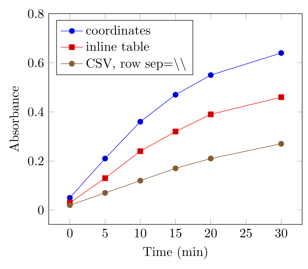
\usepackage{tikz} \usepackage{pgfplots} \pgfplotsset{compat=1.18}\begin{tikzpicture}
\begin{axis}[
xlabel={Time (min)}, ylabel={Absorbance}, ymax=0.8,
legend pos=north west, legend cell align=left,
]
% (x,y) pairs; without options each \addplot takes the next colour and mark
\addplot coordinates {
(0,0.05) (5,0.21) (10,0.36) (15,0.47) (20,0.55) (30,0.64)
};
\addlegendentry{coordinates}
% an inline table: one row per line, columns picked by their header names
\addplot table[x=t, y=A] {
t A
0 0.03
5 0.13
10 0.24
15 0.32
20 0.39
30 0.46
};
\addlegendentry{inline table}
% comma-separated values with \\ ending each row
\addplot table[col sep=comma, row sep=\\, x=t, y=A] {
t,A\\ 0,0.02\\ 5,0.07\\ 10,0.12\\ 15,0.17\\ 20,0.21\\ 30,0.27\\
};
\addlegendentry{CSV, row sep=\textbackslash\textbackslash}
\end{axis}
\end{tikzpicture}Full document
\documentclass[border=4pt]{standalone}
\usepackage{tikz}
\usepackage{pgfplots}
\pgfplotsset{compat=1.18}
\begin{document}
\begin{tikzpicture}
  \begin{axis}[
      xlabel={Time (min)}, ylabel={Absorbance}, ymax=0.8,
      legend pos=north west, legend cell align=left,
    ]
    % (x,y) pairs; without options each \addplot takes the next colour and mark
    \addplot coordinates {
      (0,0.05) (5,0.21) (10,0.36) (15,0.47) (20,0.55) (30,0.64)
    };
    \addlegendentry{coordinates}
    % an inline table: one row per line, columns picked by their header names
    \addplot table[x=t, y=A] {
      t   A
      0   0.03
      5   0.13
      10  0.24
      15  0.32
      20  0.39
      30  0.46
    };
    \addlegendentry{inline table}
    % comma-separated values with \\ ending each row
    \addplot table[col sep=comma, row sep=\\, x=t, y=A] {
      t,A\\ 0,0.02\\ 5,0.07\\ 10,0.12\\ 15,0.17\\ 20,0.21\\ 30,0.27\\
    };
    \addlegendentry{CSV, row sep=\textbackslash\textbackslash}
  \end{axis}
\end{tikzpicture}
\end{document}Scatter plots: marks coloured by a value
A scatter plot is only marks. To colour each mark by a third quantity, add scatter: the colour comes from the point’s point meta value, mapped onto the colormap from its smallest to its largest value. point meta=explicit with table[meta=age] takes it from a column; point meta=\thisrow{age} is the same, and without either, scatter colours by y. colorbar draws the scale and colorbar style={ylabel=…} labels it.
The initial colormap is hot; colormap name=viridis chooses the perceptually uniform map that, as the manual notes, also suits moderate colour blindness and greyscale printing. For groups instead of a continuous value, use scatter/classes={a={mark=*, blue}, b={mark=square*, red}} with point meta=explicit symbolic, or simply one \addplot per group with a legend entry each.
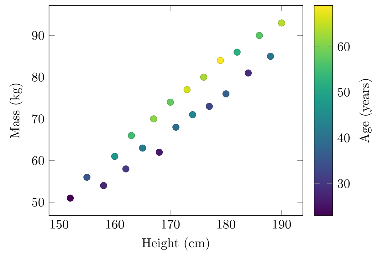
\usepackage{tikz} \usepackage{pgfplots} \pgfplotsset{compat=1.18}\begin{tikzpicture}
\begin{axis}[
xlabel={Height (cm)}, ylabel={Mass (kg)},
colormap name=viridis,
colorbar, colorbar style={ylabel={Age (years)}},
]
% scatter colours each mark by its point meta value, here the column age
\addplot[scatter, only marks, mark=*, mark size=2.5pt, point meta=explicit]
table[x=h, y=m, meta=age] {
h m age
152 51 23
155 56 35
158 54 28
160 61 47
162 58 31
163 66 55
165 63 42
167 70 61
168 62 26
170 74 58
171 68 39
173 77 66
174 71 44
176 80 63
177 73 33
179 84 69
180 76 37
182 86 52
184 81 29
186 90 57
188 85 41
190 93 64
};
\end{axis}
\end{tikzpicture}Full document
\documentclass[border=4pt]{standalone}
\usepackage{tikz}
\usepackage{pgfplots}
\pgfplotsset{compat=1.18}
\begin{document}
\begin{tikzpicture}
  \begin{axis}[
      xlabel={Height (cm)}, ylabel={Mass (kg)},
      colormap name=viridis,
      colorbar, colorbar style={ylabel={Age (years)}},
    ]
    % scatter colours each mark by its point meta value, here the column age
    \addplot[scatter, only marks, mark=*, mark size=2.5pt, point meta=explicit]
      table[x=h, y=m, meta=age] {
        h    m   age
        152  51  23
        155  56  35
        158  54  28
        160  61  47
        162  58  31
        163  66  55
        165  63  42
        167  70  61
        168  62  26
        170  74  58
        171  68  39
        173  77  66
        174  71  44
        176  80  63
        177  73  33
        179  84  69
        180  76  37
        182  86  52
        184  81  29
        186  90  57
        188  85  41
        190  93  64
      };
  \end{axis}
\end{tikzpicture}
\end{document}Error bars
Error bars are switched on per plot with error bars/.cd, followed by the direction and the source: y dir=both (or plus, minus) and y explicit to take the values from the data. In a table, y error=sd names the column (y error plus and y error minus for asymmetric errors); in a coordinate list, write (1,2) +- (0,0.3). y fixed=0.5 and y fixed relative=0.1 draw the same error for every point. x dir and x explicit do the same horizontally, and error bar style={…} and error mark change how the bars and their caps look.
Say in the legend or the caption what the bars show (standard deviation, standard error or a confidence interval) and how many replicates there are: pgfplots draws whatever numbers it is given.
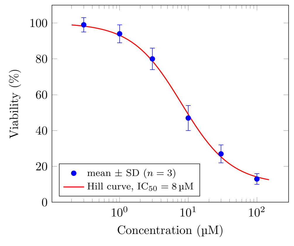
\usepackage{tikz} \usepackage{pgfplots} \pgfplotsset{compat=1.18} \usepackage{siunitx} \DeclareSIUnit{\molar}{M}\begin{tikzpicture}
\begin{semilogxaxis}[
xlabel={Concentration (\unit{\micro\molar})},
ylabel={Viability (\%)},
ymin=0, ymax=110,
legend pos=south west, legend cell align=left, legend style={font=\footnotesize},
]
% mean +- standard deviation from the columns mean and sd
\addplot[only marks, mark=*, blue,
error bars/.cd, y dir=both, y explicit]
table[x=c, y=mean, y error=sd] {
c mean sd
0.3 99 4
1 94 5
3 80 6
10 47 7
30 27 5
100 13 3
};
\addlegendentry{mean $\pm$ SD ($n = 3$)}
% a dose-response curve as an expression (on a log axis the samples are spaced logarithmically)
\addplot[red, thick, domain=0.2:150, samples=60] {10 + 90/(1 + (x/8)^1.2)};
\addlegendentry{Hill curve, $\mathrm{IC}_{50} = \qty{8}{\micro\molar}$}
\end{semilogxaxis}
\end{tikzpicture}Full document
\documentclass[border=4pt]{standalone}
\usepackage{tikz}
\usepackage{pgfplots}
\pgfplotsset{compat=1.18}
\usepackage{siunitx}
\DeclareSIUnit{\molar}{M}
\begin{document}
\begin{tikzpicture}
  \begin{semilogxaxis}[
      xlabel={Concentration (\unit{\micro\molar})},
      ylabel={Viability (\%)},
      ymin=0, ymax=110,
      legend pos=south west, legend cell align=left, legend style={font=\footnotesize},
    ]
    % mean +- standard deviation from the columns mean and sd
    \addplot[only marks, mark=*, blue,
             error bars/.cd, y dir=both, y explicit]
      table[x=c, y=mean, y error=sd] {
        c    mean  sd
        0.3  99    4
        1    94    5
        3    80    6
        10   47    7
        30   27    5
        100  13    3
      };
    \addlegendentry{mean $\pm$ SD ($n = 3$)}
    % a dose-response curve as an expression (on a log axis the samples are spaced logarithmically)
    \addplot[red, thick, domain=0.2:150, samples=60] {10 + 90/(1 + (x/8)^1.2)};
    \addlegendentry{Hill curve, $\mathrm{IC}_{50} = \qty{8}{\micro\molar}$}
  \end{semilogxaxis}
\end{tikzpicture}
\end{document}Bar charts
ybar on the axis turns every plot into vertical bars, set side by side when there are several plots; xbar makes horizontal bars, and ybar stacked stacks them. For categories, symbolic x coords={Control, Drug A, …} declares the names in order, xtick=data puts one tick under each, and the coordinates then use the names: (Drug A,82). A name that is not in the list is an error, spaces included.
bar width sets the width of each bar, enlarge x limits the space at both ends, ymin=0 makes the bars start at zero, and nodes near coords writes each value on its bar. A legend above the plot in one row is legend style={at={(0.5,1.02)}, anchor=south, legend columns=-1}.
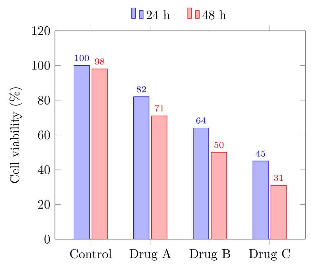
\usepackage{tikz} \usepackage{pgfplots} \pgfplotsset{compat=1.18}\begin{tikzpicture}
\begin{axis}[
ybar, bar width=12pt,
symbolic x coords={Control, Drug A, Drug B, Drug C},
xtick=data,
ymin=0, ymax=120, ylabel={Cell viability (\%)},
enlarge x limits=0.2,
nodes near coords, nodes near coords style={font=\scriptsize},
legend style={at={(0.5,1.02)}, anchor=south, legend columns=-1, draw=none,
/tikz/every even column/.append style={column sep=0.4cm}},
]
\addplot coordinates {(Control,100) (Drug A,82) (Drug B,64) (Drug C,45)};
\addplot coordinates {(Control,98) (Drug A,71) (Drug B,50) (Drug C,31)};
\legend{24 h, 48 h}
\end{axis}
\end{tikzpicture}Full document
\documentclass[border=4pt]{standalone}
\usepackage{tikz}
\usepackage{pgfplots}
\pgfplotsset{compat=1.18}
\begin{document}
\begin{tikzpicture}
  \begin{axis}[
      ybar, bar width=12pt,
      symbolic x coords={Control, Drug A, Drug B, Drug C},
      xtick=data,
      ymin=0, ymax=120, ylabel={Cell viability (\%)},
      enlarge x limits=0.2,
      nodes near coords, nodes near coords style={font=\scriptsize},
      legend style={at={(0.5,1.02)}, anchor=south, legend columns=-1, draw=none,
                    /tikz/every even column/.append style={column sep=0.4cm}},
    ]
    \addplot coordinates {(Control,100) (Drug A,82) (Drug B,64) (Drug C,45)};
    \addplot coordinates {(Control,98) (Drug A,71) (Drug B,50) (Drug C,31)};
    \legend{24 h, 48 h}
  \end{axis}
\end{tikzpicture}
\end{document}Logarithmic axes
semilogyaxis is the right axis for exponential growth or decay, which becomes a straight line; loglogaxis for power laws and frequency responses. Ticks are placed at powers of ten (log basis x=2 changes the base) and grid=both draws the minor lines for 2, 3, … 9. On a logarithmic x axis, the samples of an expression are spaced logarithmically, so the curve is smooth at both ends. Every value must be positive: zero or negative coordinates are dropped from a log axis.
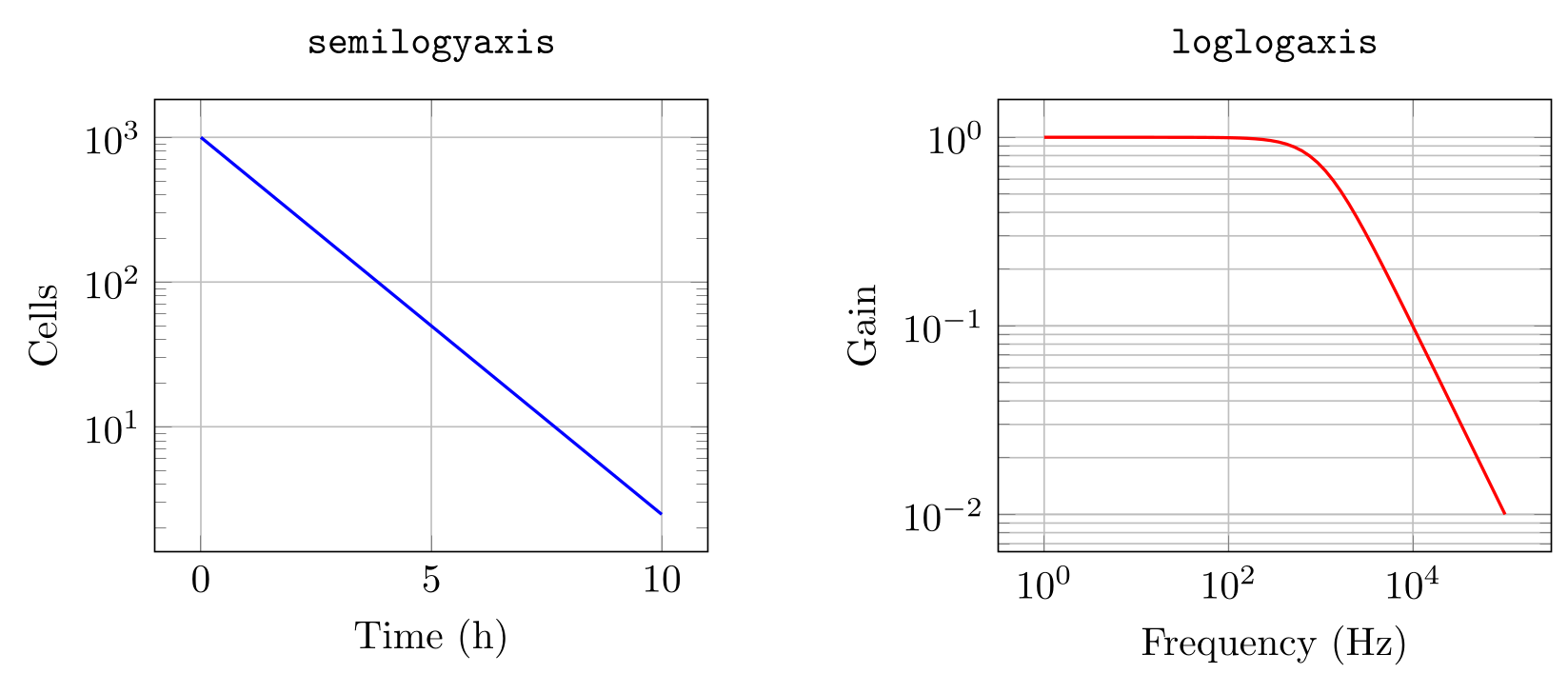
\usepackage{tikz} \usepackage{pgfplots} \pgfplotsset{compat=1.18}\begin{tikzpicture}
% logarithmic y axis: exponential decay becomes a straight line
\begin{semilogyaxis}[
width=6.5cm, title={\texttt{semilogyaxis}},
xlabel={Time (h)}, ylabel={Cells}, grid=major,
]
\addplot[blue, thick, domain=0:10] {1000*exp(-0.6*x)};
\end{semilogyaxis}
% both axes logarithmic: a first-order low-pass filter
\begin{loglogaxis}[
xshift=7.5cm, width=6.5cm, title={\texttt{loglogaxis}},
xlabel={Frequency (Hz)}, ylabel={Gain}, grid=both,
]
\addplot[red, thick, domain=1:1e5, samples=60] {1/sqrt(1 + (x/1000)^2)};
\end{loglogaxis}
\end{tikzpicture}Full document
\documentclass[border=4pt]{standalone}
\usepackage{tikz}
\usepackage{pgfplots}
\pgfplotsset{compat=1.18}
\begin{document}
\begin{tikzpicture}
  % logarithmic y axis: exponential decay becomes a straight line
  \begin{semilogyaxis}[
      width=6.5cm, title={\texttt{semilogyaxis}},
      xlabel={Time (h)}, ylabel={Cells}, grid=major,
    ]
    \addplot[blue, thick, domain=0:10] {1000*exp(-0.6*x)};
  \end{semilogyaxis}
  % both axes logarithmic: a first-order low-pass filter
  \begin{loglogaxis}[
      xshift=7.5cm, width=6.5cm, title={\texttt{loglogaxis}},
      xlabel={Frequency (Hz)}, ylabel={Gain}, grid=both,
    ]
    \addplot[red, thick, domain=1:1e5, samples=60] {1/sqrt(1 + (x/1000)^2)};
  \end{loglogaxis}
\end{tikzpicture}
\end{document}Legends, axis labels with units, and grids
- Legend.
\addlegendentry{…}after each\addplot, or\legend{a, b, c}once for all.legend pos=takesnorth west,north east(the default),south west,south eastorouter north east; anywhere else islegend style={at={(x,y)}, anchor=…}in axis-relative units (0 to 1).legend cell align=leftaligns the texts,legend columns=-1puts all entries in one row. - Units. With
\usepackage{siunitx}, writexlabel={Time (\unit{\second})}and\qty{75}{\watt}; in siunitx 3,\unitand\qtyreplace\siand\SI, which still work. A unit siunitx lacks, such as molar, is declared once:\DeclareSIUnit{\molar}{M}. pgfplots also has aunitslibrary (x unit=m, x unit prefix=k) that writes the unit in square brackets. - Grids.
grid=major,minororboth;minor tick num=1adds one minor tick between major ones;grid style={gray!25}keeps the grid behind the data visually.
Journal-ready figures: size, fonts and colour-blind-safe colours
Size. Draw the figure at the size it will be printed, so that the text in it matches the caption: a single journal column is usually 8–9 cm, a full page width 17–18 cm. width=8.5cm sets the width of the whole figure, labels included, but pgfplots only estimates the space for labels (45 pt): the example below came out 8.7 cm wide. With scale only axis, width and height apply to the axis box exactly and the labels come on top. Avoid \resizebox or \scalebox around a finished plot: they shrink or stretch the text with the drawing. Changing width and height, or scale on the axis, rescales the axis and keeps the font size.
Fonts and lines. font=\footnotesize on the axis applies to tick labels, labels and legend; tick label style={font=\scriptsize} changes one kind only. Lines are 0.4 pt by default; every axis plot/.append style={thick} makes all plotted lines 0.8 pt. To use one style for every plot in a document, put it in the preamble with \pgfplotsset{every axis/.append style={…}}.
Colours. The default cycle list uses pure blue, red and brown. For readers with colour-vision deficiency, define a palette such as Okabe–Ito with \definecolor and give it to cycle list={…}, with a different mark for each series so that the series also survive greyscale printing. The LabCanvas colour palettes page shows Okabe–Ito, Paul Tol, viridis and cividis under simulated colour blindness, with their HEX codes. For continuous values (scatter colours, surfaces), use colormap name=viridis rather than jet.
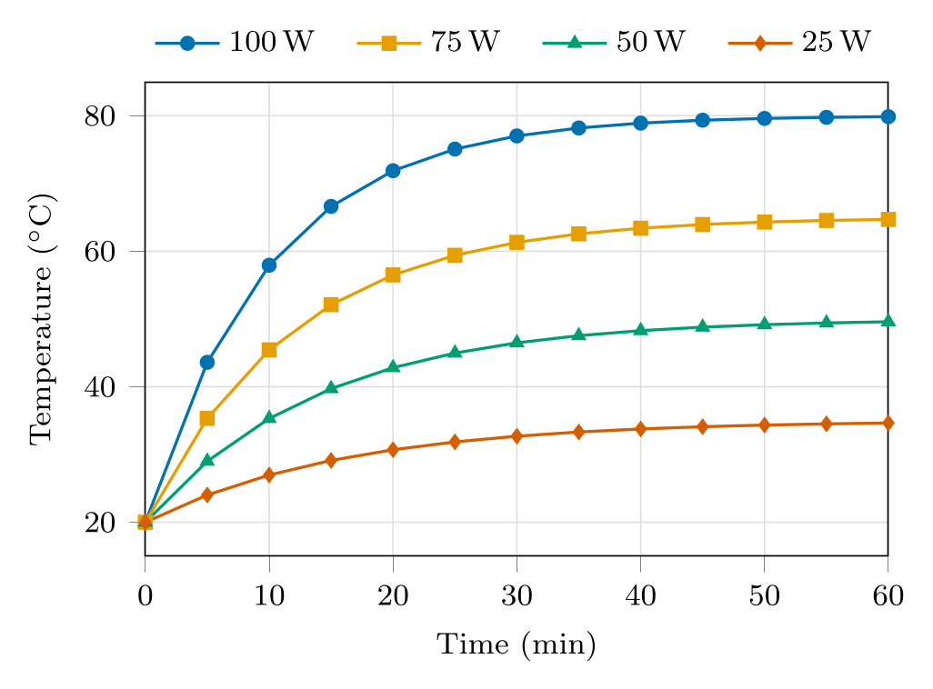
\usepackage{tikz} \usepackage{pgfplots} \pgfplotsset{compat=1.18} \usepackage{siunitx} \definecolor{oiblue}{HTML}{0072B2} \definecolor{oiorange}{HTML}{E69F00} \definecolor{oigreen}{HTML}{009E73} \definecolor{oivermillion}{HTML}{D55E00}\begin{tikzpicture}
\begin{axis}[
width=8.5cm, height=6cm, % one journal column
font=\footnotesize, % all text in the axis
xlabel={Time (\unit{\minute})},
ylabel={Temperature (\unit{\degreeCelsius})},
xmin=0, xmax=60, ymin=15, ymax=85,
grid=major, grid style={gray!25},
tick align=outside, tick pos=left,
% Okabe-Ito colours, with a different mark for each series
cycle list={
{oiblue, mark=*},
{oiorange, mark=square*},
{oigreen, mark=triangle*},
{oivermillion, mark=diamond*},
},
every axis plot/.append style={thick, mark size=1.6pt},
domain=0:60, samples=13,
legend style={at={(0.5,1.02)}, anchor=south, legend columns=-1, draw=none,
/tikz/every even column/.append style={column sep=0.3cm}},
]
\addplot {20 + 60*(1 - exp(-x/10))}; \addlegendentry{\qty{100}{\watt}}
\addplot {20 + 45*(1 - exp(-x/12))}; \addlegendentry{\qty{75}{\watt}}
\addplot {20 + 30*(1 - exp(-x/14))}; \addlegendentry{\qty{50}{\watt}}
\addplot {20 + 15*(1 - exp(-x/16))}; \addlegendentry{\qty{25}{\watt}}
\end{axis}
\end{tikzpicture}Full document
\documentclass[border=4pt]{standalone}
\usepackage{tikz}
\usepackage{pgfplots}
\pgfplotsset{compat=1.18}
\usepackage{siunitx}
\definecolor{oiblue}{HTML}{0072B2}
\definecolor{oiorange}{HTML}{E69F00}
\definecolor{oigreen}{HTML}{009E73}
\definecolor{oivermillion}{HTML}{D55E00}
\begin{document}
\begin{tikzpicture}
  \begin{axis}[
      width=8.5cm, height=6cm,        % one journal column
      font=\footnotesize,             % all text in the axis
      xlabel={Time (\unit{\minute})},
      ylabel={Temperature (\unit{\degreeCelsius})},
      xmin=0, xmax=60, ymin=15, ymax=85,
      grid=major, grid style={gray!25},
      tick align=outside, tick pos=left,
      % Okabe-Ito colours, with a different mark for each series
      cycle list={
        {oiblue, mark=*},
        {oiorange, mark=square*},
        {oigreen, mark=triangle*},
        {oivermillion, mark=diamond*},
      },
      every axis plot/.append style={thick, mark size=1.6pt},
      domain=0:60, samples=13,
      legend style={at={(0.5,1.02)}, anchor=south, legend columns=-1, draw=none,
                    /tikz/every even column/.append style={column sep=0.3cm}},
    ]
    \addplot {20 + 60*(1 - exp(-x/10))};  \addlegendentry{\qty{100}{\watt}}
    \addplot {20 + 45*(1 - exp(-x/12))};  \addlegendentry{\qty{75}{\watt}}
    \addplot {20 + 30*(1 - exp(-x/14))};  \addlegendentry{\qty{50}{\watt}}
    \addplot {20 + 15*(1 - exp(-x/16))};  \addlegendentry{\qty{25}{\watt}}
  \end{axis}
\end{tikzpicture}
\end{document}3D plots: surf, mesh, view angles and colormaps
\addplot3 takes three coordinates. With an expression in x and y, it samples a grid of samples × samples points over domain (x) and y domain (which is the same as domain if not given), and surf fills it as a coloured surface, mesh as a wireframe. Colours follow z through the colormap; shader=interp blends them smoothly, shader=flat gives each patch one colour, and the default faceted adds the grid lines.
view={⟨azimuth⟩}{⟨elevation⟩} turns the box, in degrees: the default is {25}{30}, and view={0}{90} looks straight down, which turns a surface into a heat map. Ticks at the corner shared by the x and y axes can collide, so thin them with xtick and ytick. Data from a file works as well: \addplot3[surf] table {…}; with x, y and z columns, sorted by one coordinate and with an empty line (or mesh/rows) between the scan lines. Contour plots need contour lua, which only works with LuaLaTeX, or contour gnuplot, which needs gnuplot and shell escape. Large surfaces are slow: 30 × 30 samples are 900 patches that TeX computes on every compilation.
“TikZ 3D” can also mean drawing in three dimensions without data: TikZ’s 3d library and the tikz-3dplot package handle 3D coordinates and rotated views for geometry and physics sketches.
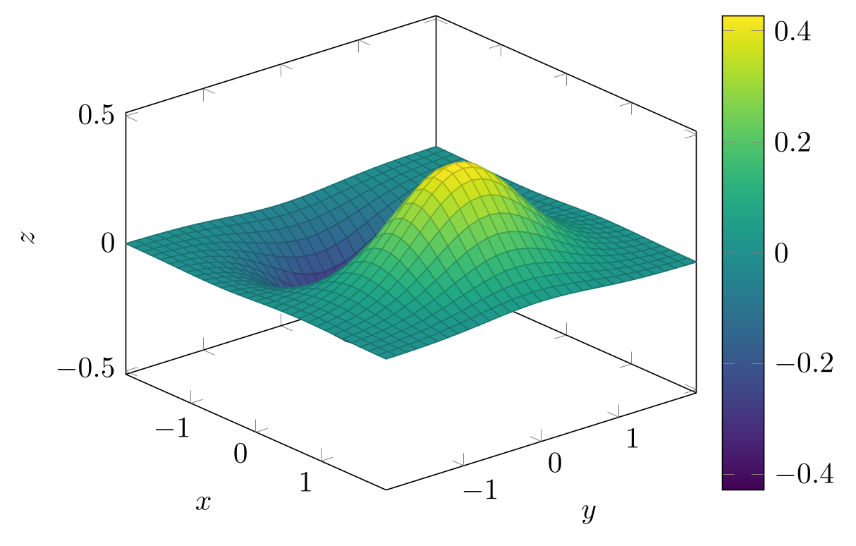
\usepackage{tikz} \usepackage{pgfplots} \pgfplotsset{compat=1.18}\begin{tikzpicture}
\begin{axis}[
view={50}{30}, % azimuth, elevation (default {25}{30})
xlabel={$x$}, ylabel={$y$}, zlabel={$z$},
xtick={-1,0,1}, ytick={-1,0,1}, % no labels at the shared front corner
colormap name=viridis, colorbar,
]
% z = f(x,y) over domain (x) and y domain (same as domain if not given)
\addplot3[surf, domain=-2:2, samples=31] {x*exp(-x^2 - y^2)};
\end{axis}
\end{tikzpicture}Full document
\documentclass[border=4pt]{standalone}
\usepackage{tikz}
\usepackage{pgfplots}
\pgfplotsset{compat=1.18}
\begin{document}
\begin{tikzpicture}
  \begin{axis}[
      view={50}{30},                 % azimuth, elevation (default {25}{30})
      xlabel={$x$}, ylabel={$y$}, zlabel={$z$},
      xtick={-1,0,1}, ytick={-1,0,1},  % no labels at the shared front corner
      colormap name=viridis, colorbar,
    ]
    % z = f(x,y) over domain (x) and y domain (same as domain if not given)
    \addplot3[surf, domain=-2:2, samples=31] {x*exp(-x^2 - y^2)};
  \end{axis}
\end{tikzpicture}
\end{document}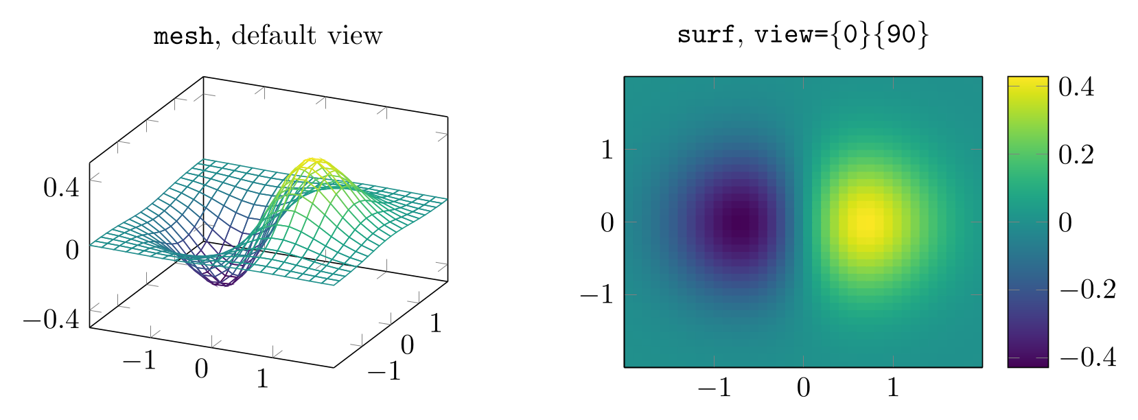
\usepackage{tikz} \usepackage{pgfplots} \pgfplotsset{compat=1.18}\begin{tikzpicture}
% a wireframe (mesh) seen from the default view={25}{30}
\begin{axis}[width=6cm, title={\texttt{mesh}, default view}, colormap name=viridis,
xtick={-1,0,1}, ytick={-1,0,1}, ztick={-0.4,0,0.4}]
\addplot3[mesh, domain=-2:2, samples=21] {x*exp(-x^2 - y^2)};
\end{axis}
% the same function seen from above: a surface becomes a heat map
\begin{axis}[xshift=6.6cm, width=6cm, title={\texttt{surf}, \texttt{view=\{0\}\{90\}}},
view={0}{90}, xtick={-1,0,1}, ytick={-1,0,1},
colormap name=viridis, colorbar]
\addplot3[surf, shader=flat, domain=-2:2, samples=41] {x*exp(-x^2 - y^2)};
\end{axis}
\end{tikzpicture}Full document
\documentclass[border=4pt]{standalone}
\usepackage{tikz}
\usepackage{pgfplots}
\pgfplotsset{compat=1.18}
\begin{document}
\begin{tikzpicture}
  % a wireframe (mesh) seen from the default view={25}{30}
  \begin{axis}[width=6cm, title={\texttt{mesh}, default view}, colormap name=viridis,
               xtick={-1,0,1}, ytick={-1,0,1}, ztick={-0.4,0,0.4}]
    \addplot3[mesh, domain=-2:2, samples=21] {x*exp(-x^2 - y^2)};
  \end{axis}
  % the same function seen from above: a surface becomes a heat map
  \begin{axis}[xshift=6.6cm, width=6cm, title={\texttt{surf}, \texttt{view=\{0\}\{90\}}},
               view={0}{90}, xtick={-1,0,1}, ytick={-1,0,1},
               colormap name=viridis, colorbar]
    \addplot3[surf, shader=flat, domain=-2:2, samples=41] {x*exp(-x^2 - y^2)};
  \end{axis}
\end{tikzpicture}
\end{document}Multi-panel figures with groupplots
For panels a, b, c… of one figure with aligned axes, load \usepgfplotslibrary{groupplots} and use a groupplot environment: group style={group size=2 by 1} sets columns by rows, and each \nextgroupplot[…] starts the next axis, with options for that panel only. Options given to groupplot itself apply to all panels, so the axes get the same size and limits. horizontal sep and vertical sep set the gaps, and y descriptions at=edge left (or x descriptions at=edge bottom) keeps the tick labels and axis label on the outer panels only. Never add more \nextgroupplot than columns × rows.
The panel letters here are titles moved to the top-left corner. To combine a pgfplots panel with a photo, a diagram or a plot from another program, export each part and assemble them in a figure editor instead (see TikZ export).
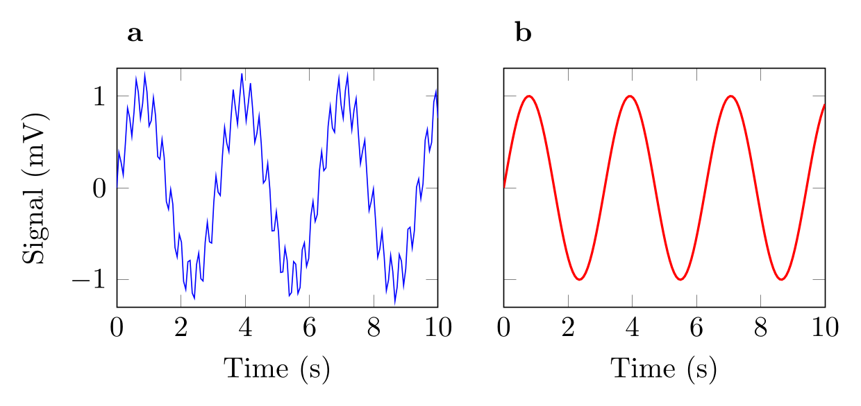
\usepackage{tikz} \usepackage{pgfplots} \pgfplotsset{compat=1.18} \usepgfplotslibrary{groupplots}\begin{tikzpicture}
\begin{groupplot}[
group style={group size=2 by 1, horizontal sep=0.8cm, y descriptions at=edge left},
width=5.5cm, height=4.5cm,
xmin=0, xmax=10, ymin=-1.3, ymax=1.3,
xlabel={Time (s)}, ylabel={Signal (mV)},
% panel letters above the top-left corner of each axis
title style={at={(0,1)}, anchor=south west, font=\bfseries},
samples=150, domain=0:10,
]
\nextgroupplot[title=a]
\addplot[blue] {sin(deg(2*x)) + 0.25*sin(deg(23*x))};
\nextgroupplot[title=b]
\addplot[red, thick] {sin(deg(2*x))};
\end{groupplot}
\end{tikzpicture}Full document
\documentclass[border=4pt]{standalone}
\usepackage{tikz}
\usepackage{pgfplots}
\pgfplotsset{compat=1.18}
\usepgfplotslibrary{groupplots}
\begin{document}
\begin{tikzpicture}
  \begin{groupplot}[
      group style={group size=2 by 1, horizontal sep=0.8cm, y descriptions at=edge left},
      width=5.5cm, height=4.5cm,
      xmin=0, xmax=10, ymin=-1.3, ymax=1.3,
      xlabel={Time (s)}, ylabel={Signal (mV)},
      % panel letters above the top-left corner of each axis
      title style={at={(0,1)}, anchor=south west, font=\bfseries},
      samples=150, domain=0:10,
    ]
    \nextgroupplot[title=a]
      \addplot[blue] {sin(deg(2*x)) + 0.25*sin(deg(23*x))};
    \nextgroupplot[title=b]
      \addplot[red, thick] {sin(deg(2*x))};
  \end{groupplot}
\end{tikzpicture}
\end{document}Plain TikZ plot: functions without pgfplots
TikZ itself can plot: \draw[domain=0:6.28, samples=100, smooth, variable=\x] plot ({\x}, {sin(\x r)}); draws a curve in the picture’s own coordinates, and plot coordinates {(1,0.3) (2,1.1)} draws given points (only marks for markers). The r after a number tells TikZ that it is in radians. There are no automatic axes, ticks or legend: you draw them yourself, as below, which suits a small sketch in a diagram. Plain TikZ also computes with TeX dimensions, so a value beyond about 16 000 stops with Dimension too large; pgfplots computes in floating point and scales the axis for you.
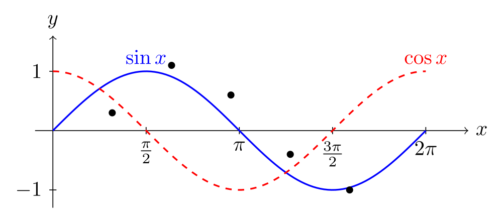
\usepackage{tikz}\begin{tikzpicture}
% axes are ordinary lines: plain TikZ draws no ticks or labels for you
\draw[->] (-0.3,0) -- (7,0) node[right] {$x$};
\draw[->] (0,-1.3) -- (0,1.6) node[above] {$y$};
\foreach \x/\label in {1.5708/\frac{\pi}{2}, 3.1416/\pi, 4.7124/\frac{3\pi}{2}, 6.2832/2\pi}
\draw (\x,0.06) -- (\x,-0.06) node[below] {$\label$};
\foreach \y in {-1, 1}
\draw (0.06,\y) -- (-0.06,\y) node[left] {$\y$};
% plot (x, f(x)) for x in the domain; sin and cos take degrees, so r converts radians
\draw[blue, thick, domain=0:6.2832, samples=100, smooth, variable=\x]
plot ({\x}, {sin(\x r)});
\draw[red, thick, dashed, domain=0:6.2832, samples=100, smooth, variable=\x]
plot ({\x}, {cos(\x r)});
\node[blue, above] at (1.5708,1) {$\sin x$};
\node[red, above] at (6.2832,1) {$\cos x$};
% points given inline, drawn as marks only
\draw plot[only marks, mark=*, mark size=1.5pt] coordinates {(1,0.3) (2,1.1) (3,0.6) (4,-0.4) (5,-1)};
\end{tikzpicture}Full document
\documentclass[border=4pt]{standalone}
\usepackage{tikz}
\begin{document}
\begin{tikzpicture}
  % axes are ordinary lines: plain TikZ draws no ticks or labels for you
  \draw[->] (-0.3,0) -- (7,0) node[right] {$x$};
  \draw[->] (0,-1.3) -- (0,1.6) node[above] {$y$};
  \foreach \x/\label in {1.5708/\frac{\pi}{2}, 3.1416/\pi, 4.7124/\frac{3\pi}{2}, 6.2832/2\pi}
    \draw (\x,0.06) -- (\x,-0.06) node[below] {$\label$};
  \foreach \y in {-1, 1}
    \draw (0.06,\y) -- (-0.06,\y) node[left] {$\y$};
  % plot (x, f(x)) for x in the domain; sin and cos take degrees, so r converts radians
  \draw[blue, thick, domain=0:6.2832, samples=100, smooth, variable=\x]
    plot ({\x}, {sin(\x r)});
  \draw[red, thick, dashed, domain=0:6.2832, samples=100, smooth, variable=\x]
    plot ({\x}, {cos(\x r)});
  \node[blue, above] at (1.5708,1) {$\sin x$};
  \node[red, above] at (6.2832,1) {$\cos x$};
  % points given inline, drawn as marks only
  \draw plot[only marks, mark=*, mark size=1.5pt] coordinates {(1,0.3) (2,1.1) (3,0.6) (4,-0.4) (5,-1)};
\end{tikzpicture}
\end{document}Plots made in Python, MATLAB or a statistics program
If the plot already exists in matplotlib or MATLAB, converters write pgfplots code for it: tikzplotlib and its maintained fork matplot2tikz for matplotlib, matlab2tikz for MATLAB. Their status and output are on the export page. Often the cleaner route is to export the data as CSV and plot it with \addplot table, as above.
pgfplots draws; it does not do statistics. For t tests, ANOVA, curve fitting with confidence bands or survival curves, a tool such as LabCanvas Graphs is easier: it fits and tests the data and draws the plot from the same table.
Common errors and how to fix them
| LaTeX says (or you see) | Cause and fix |
|---|---|
| Package pgfplots Warning: running in backwards compatibility mode (unsuitable tick labels; missing features). Consider writing \pgfplotsset{compat=1.18} into your preamble. | Add \pgfplotsset{compat=1.18} after \usepackage{pgfplots}. Without it, pgfplots imitates version 1.3, with older label placement and without newer features. |
| Package pgfplots Error: Sorry, 'compat=1.19' is unknown in this context. Please use at most 'compat=1.18'. | There is no compat level above 1.18, even in pgfplots 1.18.3: compat follows the feature set, not the package version. Write compat=1.18. |
| Environment axis undefined. | pgfplots is not loaded: add \usepackage{pgfplots} (it loads TikZ) and \pgfplotsset{compat=1.18} to the preamble. |
| Environment groupplot undefined. | groupplot is in a pgfplots library: add \usepgfplotslibrary{groupplots} after \usepackage{pgfplots}. |
| Package pgfplots Error: Could not read table file 'data.csv' in 'search path=.'. In case you intended to provide inline data: maybe TeX screwed up your end-of-lines? Try `row sep=crcr' and terminate your lines with `\\' (refer to the pgfplotstable manual for details). | The file is not where LaTeX looks: paths are relative to the main .tex file, and on Overleaf the file must be uploaded to the project. If you meant inline data inside a macro, end each row with \\ and add row sep=\\. |
| Package pgfplots Error: Sorry, could not retrieve column 't' from table '…'. Please check spelling (or introduce name aliases). | x= or y= names a column that is not in the header row. Check the spelling and case; for comma-separated data add col sep=comma, otherwise the whole line t,A is read as a single column name. |
| Package pgfplots Error: Sorry, the input coordinate `Drug B' has not been defined with 'symbolic x coords={Control, Drug A}... Maybe it has been misspelled? | Every category used in a coordinate must be listed in symbolic x coords, spelled exactly the same, spaces included. |
| Dimension too large. | A plain TikZ plot produced a value beyond TeX’s limit of about 16 000 (here exp(x) up to x = 10). Use pgfplots, which computes in floating point and scales the axis, or rescale the function. |
| File ended while scanning use of \pgfplots@addplotimpl@expression@curly. | An \addplot {…} without its closing semicolon. Every \addplot ends with ;. |
| Undefined control sequence. (in \unit{\micro\molar}) | siunitx 3 defines no \molar. Declare it once in the preamble: \DeclareSIUnit{\molar}{M}. |
| sin(x) is almost a straight line (no error) | Trigonometric functions take degrees in TikZ and pgfplots. Write sin(deg(x)), or add trig format plots=rad to the plot or axis; in plain TikZ, write sin(\x r). |
| The error bars do not appear (no error) | Both the direction and the source are needed: error bars/.cd, y dir=both, y explicit, plus y error=column in the table (or +- (0,err) in coordinates). |
Frequently asked questions
How do I plot a function in LaTeX with TikZ?
Use pgfplots: \usepackage{pgfplots} and \pgfplotsset{compat=1.18} in the preamble, then \begin{tikzpicture}\begin{axis}[xlabel=$x$, ylabel=$y$] \addplot[domain=-2:2, samples=100] {x^2}; \end{axis}\end{tikzpicture}. Remember that sin and cos take degrees: write sin(deg(x)). Plain TikZ can also draw \draw plot ({\x}, {\x^2}); but without automatic axes.
How do I make a scatter plot in TikZ?
Add only marks to the plot: \addplot[only marks, mark=*] table {data.dat}; or with coordinates {(1,2) (3,4)}. To colour the points by a third value, add scatter and point meta=explicit with table[x=…, y=…, meta=…], plus colorbar on the axis.
How do I plot data from a CSV file with pgfplots?
Write \addplot table[col sep=comma, x=time, y=value] {data.csv}; where time and value are names in the header row. The path is relative to the main .tex file. For several columns, use one \addplot per column, and y expr=\thisrow{value}*100 to scale a column.
How do I draw a 3D surface plot in TikZ?
With pgfplots: \begin{axis}[view={50}{30}, colormap name=viridis] \addplot3[surf, domain=-2:2, samples=30] {exp(-x^2-y^2)}; \end{axis}. mesh draws a wireframe instead, view={0}{90} looks from above, and colorbar adds the colour scale.
Which compat setting should I use for pgfplots?
compat=1.18, the newest level in pgfplots 1.18.3 (2026). Setting it removes the backwards-compatibility warning and gives the current label placement; a fixed number rather than compat=newest keeps old figures unchanged when pgfplots gets a new level.
Can I convert a matplotlib or MATLAB figure to TikZ?
Yes: tikzplotlib or its maintained fork matplot2tikz for matplotlib, and matlab2tikz for MATLAB, write pgfplots code that you then edit. The TikZ export page has their current status and what their output looks like; exporting the data as CSV and plotting it with \addplot table often gives cleaner code.
References
- pgfplots package on CTAN (v1.18.3)ctan.org
- pgfplots manual 1.18.3 (PDF on CTAN, 2026-08-26)mirrors.ctan.org
- pgfplots manual, §4.2 The Axis Environmentstikz.dev
- pgfplots manual, §4.3.1 Coordinate Lists and §4.3.2 Reading Coordinates From Tablestikz.dev
- pgfplots manual, §4.3.3 Computing Coordinates with Mathematical Expressions (domain, samples, trig format plots)tikz.dev
- pgfplots manual, §4.5.4 Bar Plotstikz.dev
- pgfplots manual, §4.5.12 Scatter Plotstikz.dev
- pgfplots manual, §4.6.5 Mesh Plots and §4.6.6 Surface Plotstikz.dev
- pgfplots manual, §4.6.8 Contour Plots (contour lua, contour gnuplot)tikz.dev
- pgfplots manual, §4.7.4 Font Size and Line Widthtikz.dev
- pgfplots manual, §4.7.6 Color Maps (viridis)tikz.dev
- pgfplots manual, §4.7.7 Cycle Liststikz.dev
- pgfplots manual, §4.9.4 Legends and §4.9.5 Legend Appearancetikz.dev
- pgfplots manual, §4.9.13 Color Barstikz.dev
- pgfplots manual, §4.10.1 Common Scaling Options (width, height, scale only axis)tikz.dev
- pgfplots manual, §4.11.1 View Configurationtikz.dev
- pgfplots manual, §4.12 Error Barstikz.dev
- pgfplots manual, §4.16 Grid Optionstikz.dev
- pgfplots manual, §4.21.1 String Symbols as Input Coordinates (symbolic x coords)tikz.dev
- pgfplots manual, §5.8 Grouping plots (groupplots library)tikz.dev
- pgfplots manual, §5.14 Units in Labels (units library)tikz.dev
- PGF/TikZ manual, §22.5 Plotting a Function (the plot operation)tikz.dev
- siunitx package on CTAN (v3.6.7): \unit, \qty and \DeclareSIUnitctan.org
- Okabe and Ito, Color Universal Design (colour-blind-safe palette)jfly.uni-koeln.de
The facts on this page were checked against these sources, and every picture is the code with it typeset with TeX Live 2026. Code on this page: CC0 1.0, copy it freely.
Try the code in your browserEvery snippet on this page opens in the free TikZ editor: it is typeset with TeX Live as you type, with errors pointed at their line.
Open the TikZ editor