TikZ-Feynman: Feynman diagrams in LaTeX
Quick answer
\usepackage[compat=1.1.0]{tikz-feynman}, then inside \begin{tikzpicture}\begin{feynman} … \end{feynman}\end{tikzpicture} place the vertices with \vertex (a); and \vertex [right=of a] (b); (contents in braces make an external particle label) and connect them with \diagram* { (a) -- [fermion] (b), … };. The style on each edge sets the propagator: fermion, anti fermion, photon, gluon, scalar, ghost, charged boson; edge label= and momentum= annotate it. This manual placement works with pdfLaTeX. The shorter \feynmandiagram, which places the vertices by itself, needs LuaLaTeX; under pdfLaTeX it falls back to a basic placement that usually overlaps.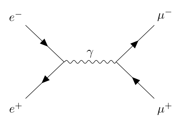
\usepackage{tikz} \usepackage[compat=1.1.0]{tikz-feynman}\begin{tikzpicture}
\begin{feynman}
\vertex (a);
\vertex [right=of a] (b);
\vertex [above left=of a] (i1) {\(e^{-}\)};
\vertex [below left=of a] (i2) {\(e^{+}\)};
\vertex [above right=of b] (f1) {\(\mu^{-}\)};
\vertex [below right=of b] (f2) {\(\mu^{+}\)};
\diagram* {
(i1) -- [fermion] (a) -- [fermion] (i2),
(a) -- [photon, edge label=\(\gamma\)] (b),
(f2) -- [fermion] (b) -- [fermion] (f1),
};
\end{feynman}
\end{tikzpicture}Full document
\documentclass[border=4pt]{standalone}
\usepackage{tikz}
\usepackage[compat=1.1.0]{tikz-feynman}
\begin{document}
\begin{tikzpicture}
  \begin{feynman}
    \vertex (a);
    \vertex [right=of a] (b);
    \vertex [above left=of a] (i1) {\(e^{-}\)};
    \vertex [below left=of a] (i2) {\(e^{+}\)};
    \vertex [above right=of b] (f1) {\(\mu^{-}\)};
    \vertex [below right=of b] (f2) {\(\mu^{+}\)};
    \diagram* {
      (i1) -- [fermion] (a) -- [fermion] (i2),
      (a) -- [photon, edge label=\(\gamma\)] (b),
      (f2) -- [fermion] (b) -- [fermion] (f1),
    };
  \end{feynman}
\end{tikzpicture}
\end{document}Contents
Loading TikZ-Feynman, and its status in 2026
TikZ-Feynman, by Joshua Ellis, is on CTAN and in TeX Live and MiKTeX. Its current version is still 1.1.0 of 5 February 2016: there has been no release since, the main branch of the GitHub repository last changed in April 2018, and the 2023 commits on its development branch only touch the build and tests. The package nevertheless works on current TeX Live: every picture on this page was compiled with TeX Live 2026 and PGF 3.1.12, with pdfLaTeX for manual placement and LuaLaTeX for the automatic layouts. (The Lua patches it ships are applied only for the old PGF versions 3.0.0 and 3.0.1, so current PGF runs it unpatched.)
Load it as the manual recommends, with the version you wrote for: \usepackage[compat=1.1.0]{tikz-feynman}.
Without compat it warns “Consider loading TikZ-Feynman with \usepackage[compat=1.1.0]{tikz-feynman} so that you can be warned if TikZ-Feynman changes.” The package loads TikZ and the libraries it needs (positioning, decorations.markings, decorations.pathmorphing, graphs, patterns, shapes.geometric and, under LuaLaTeX only, graphdrawing with the force, layered, trees and circular algorithms). If you use it in a paper, the author asks you to cite arXiv:1601.05437.
Manual placement: \vertex and \diagram*
Manual placement is the reliable method and the one that works with pdfLaTeX (Overleaf’s default):
- The environment.
\vertexand\diagramexist only inside\begin{feynman} … \end{feynman}, which itself goes inside atikzpicture. Ordinary TikZ commands (\draw,\node) still work around it. - Vertices.
\vertex (a);is a point of zero size. Position it with coordinates,\vertex (b) at (2,0);, or relative to another vertex with the positioning library,\vertex [above right=of b] (f1);(the default distance is 1.5 cm, set by the defaultmediumsize;smallmakes it 1 cm,large2 cm, andright=2.5cm of asets one distance). Text in braces,\vertex (f1) {\(\mu^{-}\)};, turns the vertex into an external particle label. Every\vertexneeds its final semicolon, and it cannot be chained like\node. - Edges.
\diagram* { … };connects existing vertices, written in parentheses:(a) -- [fermion] (b) -- [photon] (c), (c) -- [fermion] (d). A comma ends a chain.{[edges=fermion] (a) -- (b) -- (c)}gives a whole group the same style.
Use \diagram*, with the star, for pre-placed vertices: the unstarred \diagram runs a layout algorithm, and under LuaLaTeX it stops with “attempting to create edge between nodes that are not in the graph”.
Propagator styles: fermion, photon, gluon, scalar, ghost
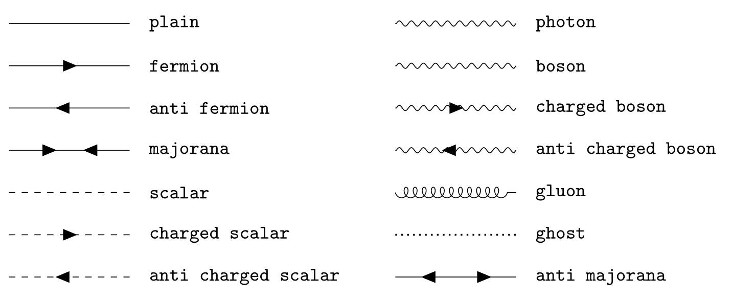
Each edge style draws one kind of line (manual §3.2.4). Styles stack, so [plain, gluon] is a gluon drawn over a straight line, as used for gluinos.
| Style | Line | Typical particle |
|---|---|---|
plain | Solid line (also the default with no style) | — |
fermion, anti fermion | Solid line with an arrow along / against the edge | electron, quark; positron, antiquark |
majorana, anti majorana | Two arrows pointing in / out | Majorana fermion |
photon, boson | Sine wave (the two are drawn the same) | γ, Z |
charged boson, anti charged boson | Sine wave with an arrow | W± |
gluon | Coils | gluon |
scalar, charged scalar, anti charged scalar | Dashed, with or without an arrow | Higgs, pion, squark |
ghost | Dotted | Faddeev–Popov ghost |
Arrow direction follows the order in which you write the edge: for an antiparticle either reverse the order or use anti fermion. Ordinary TikZ keys work on edges too: red, very thick, opacity=0.3, draw=none (an invisible edge).
\usepackage{tikz} \usepackage[compat=1.1.0]{tikz-feynman}\begin{tikzpicture}[every node/.style={font=\ttfamily\small}]
\begin{feynman}
\vertex (a1) at (0, 0); \vertex (b1) at (2, 0);
\vertex (a2) at (0,-0.7); \vertex (b2) at (2,-0.7);
\vertex (a3) at (0,-1.4); \vertex (b3) at (2,-1.4);
\vertex (a4) at (0,-2.1); \vertex (b4) at (2,-2.1);
\vertex (a5) at (0,-2.8); \vertex (b5) at (2,-2.8);
\vertex (a6) at (0,-3.5); \vertex (b6) at (2,-3.5);
\vertex (a7) at (0,-4.2); \vertex (b7) at (2,-4.2);
\vertex (c1) at (6.4, 0); \vertex (d1) at (8.4, 0);
\vertex (c2) at (6.4,-0.7); \vertex (d2) at (8.4,-0.7);
\vertex (c3) at (6.4,-1.4); \vertex (d3) at (8.4,-1.4);
\vertex (c4) at (6.4,-2.1); \vertex (d4) at (8.4,-2.1);
\vertex (c5) at (6.4,-2.8); \vertex (d5) at (8.4,-2.8);
\vertex (c6) at (6.4,-3.5); \vertex (d6) at (8.4,-3.5);
\vertex (c7) at (6.4,-4.2); \vertex (d7) at (8.4,-4.2);
\diagram* {
(a1) -- [plain] (b1), (c1) -- [photon] (d1),
(a2) -- [fermion] (b2), (c2) -- [boson] (d2),
(a3) -- [anti fermion] (b3), (c3) -- [charged boson] (d3),
(a4) -- [majorana] (b4), (c4) -- [anti charged boson] (d4),
(a5) -- [scalar] (b5), (c5) -- [gluon] (d5),
(a6) -- [charged scalar] (b6), (c6) -- [ghost] (d6),
(a7) -- [anti charged scalar] (b7), (c7) -- [anti majorana] (d7),
};
\end{feynman}
\foreach \s [count=\i] in {plain, fermion, anti fermion, majorana, scalar, charged scalar, anti charged scalar}
\node [anchor=west] at (2.2, {-0.7*(\i-1)}) {\s};
\foreach \s [count=\i] in {photon, boson, charged boson, anti charged boson, gluon, ghost, anti majorana}
\node [anchor=west] at (8.6, {-0.7*(\i-1)}) {\s};
\end{tikzpicture}Full document
\documentclass[border=4pt]{standalone}
\usepackage{tikz}
\usepackage[compat=1.1.0]{tikz-feynman}
\begin{document}
\begin{tikzpicture}[every node/.style={font=\ttfamily\small}]
  \begin{feynman}
    \vertex (a1) at (0, 0);    \vertex (b1) at (2, 0);
    \vertex (a2) at (0,-0.7);  \vertex (b2) at (2,-0.7);
    \vertex (a3) at (0,-1.4);  \vertex (b3) at (2,-1.4);
    \vertex (a4) at (0,-2.1);  \vertex (b4) at (2,-2.1);
    \vertex (a5) at (0,-2.8);  \vertex (b5) at (2,-2.8);
    \vertex (a6) at (0,-3.5);  \vertex (b6) at (2,-3.5);
    \vertex (a7) at (0,-4.2);  \vertex (b7) at (2,-4.2);
    \vertex (c1) at (6.4, 0);    \vertex (d1) at (8.4, 0);
    \vertex (c2) at (6.4,-0.7);  \vertex (d2) at (8.4,-0.7);
    \vertex (c3) at (6.4,-1.4);  \vertex (d3) at (8.4,-1.4);
    \vertex (c4) at (6.4,-2.1);  \vertex (d4) at (8.4,-2.1);
    \vertex (c5) at (6.4,-2.8);  \vertex (d5) at (8.4,-2.8);
    \vertex (c6) at (6.4,-3.5);  \vertex (d6) at (8.4,-3.5);
    \vertex (c7) at (6.4,-4.2);  \vertex (d7) at (8.4,-4.2);
    \diagram* {
      (a1) -- [plain] (b1),            (c1) -- [photon] (d1),
      (a2) -- [fermion] (b2),          (c2) -- [boson] (d2),
      (a3) -- [anti fermion] (b3),     (c3) -- [charged boson] (d3),
      (a4) -- [majorana] (b4),         (c4) -- [anti charged boson] (d4),
      (a5) -- [scalar] (b5),           (c5) -- [gluon] (d5),
      (a6) -- [charged scalar] (b6),   (c6) -- [ghost] (d6),
      (a7) -- [anti charged scalar] (b7), (c7) -- [anti majorana] (d7),
    };
  \end{feynman}
  \foreach \s [count=\i] in {plain, fermion, anti fermion, majorana, scalar, charged scalar, anti charged scalar}
    \node [anchor=west] at (2.2, {-0.7*(\i-1)}) {\s};
  \foreach \s [count=\i] in {photon, boson, charged boson, anti charged boson, gluon, ghost, anti majorana}
    \node [anchor=west] at (8.6, {-0.7*(\i-1)}) {\s};
\end{tikzpicture}
\end{document}Vertex styles: dot, blob and particle labels
A vertex can carry a shape: dot, square dot, empty dot, crossed dot and blob (a hatched disc for an effective vertex or form factor). With \vertex, a shape is drawn only if the vertex has contents, so write the empty braces: \vertex [dot] (v) at (1,0) {};. Without {} the vertex stays a coordinate and nothing appears. Inside an automatic \diagram the shape goes after the vertex name, b [dot], and a label is i1 [particle=\(e^{-}\)]. Labels that contain a comma or brackets must be braced, particle={\(\gamma, Z\)}, and particle belongs on external vertices only (on an internal vertex it leaves a gap in the lines).

\usepackage{tikz} \usepackage[compat=1.1.0]{tikz-feynman}\begin{tikzpicture}
\begin{feynman}
% a vertex style is only drawn if the vertex has contents: note the {}
\vertex [dot] (v1) at (0, 0) {};
\vertex [square dot] (v2) at (2, 0) {};
\vertex [empty dot] (v3) at (4, 0) {};
\vertex [crossed dot] (v4) at (6, 0) {};
\vertex [blob] (v5) at (8.2, 0) {};
\vertex (l1) at (-1, 0); \vertex (r5) at (9.4, 0);
\diagram* {
(l1) -- [fermion] (v1) -- [fermion] (v2) -- [fermion] (v3)
-- [fermion] (v4) -- [fermion] (v5) -- [fermion] (r5),
};
\end{feynman}
\foreach \s/\x in {dot/0, square dot/2, empty dot/4, crossed dot/6, blob/8.2}
\node [below=0.55cm, font=\ttfamily\small] at (\x, 0) {\s};
\end{tikzpicture}Full document
\documentclass[border=4pt]{standalone}
\usepackage{tikz}
\usepackage[compat=1.1.0]{tikz-feynman}
\begin{document}
\begin{tikzpicture}
  \begin{feynman}
    % a vertex style is only drawn if the vertex has contents: note the {}
    \vertex [dot]         (v1) at (0, 0) {};
    \vertex [square dot]  (v2) at (2, 0) {};
    \vertex [empty dot]   (v3) at (4, 0) {};
    \vertex [crossed dot] (v4) at (6, 0) {};
    \vertex [blob]        (v5) at (8.2, 0) {};
    \vertex (l1) at (-1, 0);  \vertex (r5) at (9.4, 0);
    \diagram* {
      (l1) -- [fermion] (v1) -- [fermion] (v2) -- [fermion] (v3)
           -- [fermion] (v4) -- [fermion] (v5) -- [fermion] (r5),
    };
  \end{feynman}
  \foreach \s/\x in {dot/0, square dot/2, empty dot/4, crossed dot/6, blob/8.2}
    \node [below=0.55cm, font=\ttfamily\small] at (\x, 0) {\s};
\end{tikzpicture}
\end{document}Labels, momentum arrows and insertions
edge label=\(\gamma\)writes a label at the middle of the edge, on the left of the direction of travel;edge label'=…on the right.momentum=\(p\)draws an arrow with a label parallel to the edge;momentum'=puts it on the other side;reversed momentum=(aliasrmomentum) andreversed momentum'=point it the other way.- Momentum arrows do not inherit the edge’s colour: style them in an optional argument,
momentum={[arrow style=red, label style=red]\(k\)}.arrow distance(3 mm),arrow shorten(0.15) andlabel distanceadjust the arrow (manual §3.2.5). insertion=0.5puts a cross on the edge at that fraction of its length, for a mass or momentum insertion; repeat the key for several.
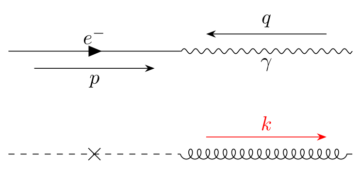
\usepackage{tikz} \usepackage[compat=1.1.0]{tikz-feynman}\begin{tikzpicture}
\begin{feynman}
\vertex (a) at (0, 0); \vertex (b) at (3, 0); \vertex (c) at (6, 0);
\vertex (d) at (0,-1.8); \vertex (e) at (3,-1.8); \vertex (f) at (6,-1.8);
\diagram* {
(a) -- [fermion, edge label=\(e^{-}\), momentum'=\(p\)] (b)
-- [photon, edge label'=\(\gamma\), reversed momentum=\(q\)] (c),
(d) -- [scalar, insertion=0.5] (e)
-- [gluon, momentum={[arrow style=red, label style=red]\(k\)}] (f),
};
\end{feynman}
\end{tikzpicture}Full document
\documentclass[border=4pt]{standalone}
\usepackage{tikz}
\usepackage[compat=1.1.0]{tikz-feynman}
\begin{document}
\begin{tikzpicture}
  \begin{feynman}
    \vertex (a) at (0, 0);    \vertex (b) at (3, 0);    \vertex (c) at (6, 0);
    \vertex (d) at (0,-1.8);  \vertex (e) at (3,-1.8);  \vertex (f) at (6,-1.8);
    \diagram* {
      (a) -- [fermion, edge label=\(e^{-}\), momentum'=\(p\)] (b)
          -- [photon, edge label'=\(\gamma\), reversed momentum=\(q\)] (c),
      (d) -- [scalar, insertion=0.5] (e)
          -- [gluon, momentum={[arrow style=red, label style=red]\(k\)}] (f),
    };
  \end{feynman}
\end{tikzpicture}
\end{document}Automatic layout with LuaLaTeX
Without positions, \diagram (or the shorthand \feynmandiagram [options] {…};, which creates the tikzpicture and feynman environments for you) hands the vertices to the TikZ graph drawing algorithms, which are written in Lua and therefore need LuaLaTeX. Name the vertices freely; a name used twice is the same vertex. horizontal=a to b rotates the result so that a and b are on a horizontal line (horizontal' mirrors it, vertical works the same way), and small, medium (default) and large set the spacing.
Under pdfLaTeX the same code still compiles, with the warning “Package tikz-feynman Warning: LuaTeX is required if you wish to have vertices automatically placed.” and a rudimentary placement in which vertices and labels pile up. Layout keys such as layered layout are then silently ignored. Either switch the engine (lualatex file.tex; on Overleaf, choose LuaLaTeX as the compiler in the project menu) or place the vertices by hand as above. The spring layout decides which side each particle ends up on, so the same diagram can come out mirrored compared with a manual drawing (here e+ is on top).
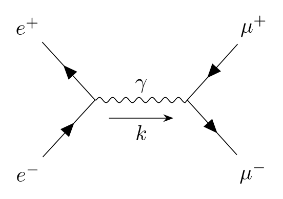
\usepackage{tikz} \usepackage[compat=1.1.0]{tikz-feynman}Compile with LuaLaTeX\begin{tikzpicture}
\begin{feynman}
% no positions: the spring layout places the vertices (LuaLaTeX only)
\diagram [horizontal=a to b] {
i1 [particle=\(e^{-}\)] -- [fermion] a -- [fermion] i2 [particle=\(e^{+}\)],
a -- [photon, edge label=\(\gamma\), momentum'=\(k\)] b,
f1 [particle=\(\mu^{+}\)] -- [fermion] b -- [fermion] f2 [particle=\(\mu^{-}\)],
};
\end{feynman}
\end{tikzpicture}Full document
\documentclass[border=4pt]{standalone}
\usepackage{tikz}
\usepackage[compat=1.1.0]{tikz-feynman}
\begin{document}
\begin{tikzpicture}
  \begin{feynman}
    % no positions: the spring layout places the vertices (LuaLaTeX only)
    \diagram [horizontal=a to b] {
      i1 [particle=\(e^{-}\)] -- [fermion] a -- [fermion] i2 [particle=\(e^{+}\)],
      a -- [photon, edge label=\(\gamma\), momentum'=\(k\)] b,
      f1 [particle=\(\mu^{+}\)] -- [fermion] b -- [fermion] f2 [particle=\(\mu^{-}\)],
    };
  \end{feynman}
\end{tikzpicture}
\end{document}Choosing a layout algorithm
The default spring layout spreads vertices out evenly, which suits scattering diagrams. For decays, with one particle on the left and the products on the right, use layered layout: the first vertex of each edge is put on the layer before the second, so the order in which you write edges matters (c -- f2, c -- f3 puts both f’s after c; f2 -- c -- f3 does not). tree layout, spring electrical layout and the key same layer are also available, and an invisible edge (draw=none) pulls two vertices together without drawing anything. When none of these gives the picture you want, place the vertices by hand.
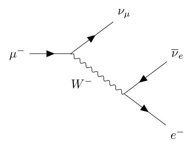
\usepackage{tikz} \usepackage[compat=1.1.0]{tikz-feynman}Compile with LuaLaTeX\begin{tikzpicture}
\begin{feynman}
% layered layout: the first vertex of each edge goes on the layer before the second
\diagram [layered layout, horizontal=a to b] {
a [particle=\(\mu^{-}\)] -- [fermion] b -- [fermion] f1 [particle=\(\nu_{\mu}\)],
b -- [boson, edge label'=\(W^{-}\)] c,
c -- [anti fermion] f2 [particle=\(\overline{\nu}_{e}\)],
c -- [fermion] f3 [particle=\(e^{-}\)],
};
\end{feynman}
\end{tikzpicture}Full document
\documentclass[border=4pt]{standalone}
\usepackage{tikz}
\usepackage[compat=1.1.0]{tikz-feynman}
\begin{document}
\begin{tikzpicture}
  \begin{feynman}
    % layered layout: the first vertex of each edge goes on the layer before the second
    \diagram [layered layout, horizontal=a to b] {
      a [particle=\(\mu^{-}\)] -- [fermion] b -- [fermion] f1 [particle=\(\nu_{\mu}\)],
      b -- [boson, edge label'=\(W^{-}\)] c,
      c -- [anti fermion] f2 [particle=\(\overline{\nu}_{e}\)],
      c -- [fermion] f3 [particle=\(e^{-}\)],
    };
  \end{feynman}
\end{tikzpicture}
\end{document}Classic diagrams: Compton scattering, a loop and gluon fusion
Compton scattering (e−γ → e−γ) has two tree-level diagrams: in the s-channel the electron absorbs the photon before emitting one, in the u-channel it emits first, so the photon lines cross. Both are the same electron line with the photons attached to the other vertex.
Loops use the modifier keys half left and half right (half circles), quarter left and quarter right, or TikZ’s out=, in=, bend left and looseness= for any curve. The photon self-energy below runs (b) -- [fermion, half left] (c) -- [fermion, half left] (b), which closes the loop with consistent fermion arrows.
Gluon fusion to a Higgs boson (gg → H through a top-quark loop) combines gluon, fermion and scalar lines; the triangle is three fermion edges in a closed chain.
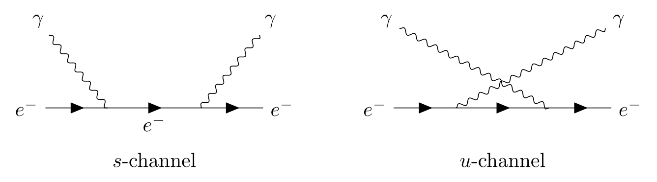
\usepackage{tikz} \usepackage[compat=1.1.0]{tikz-feynman}\begin{tikzpicture}
\begin{feynman}
% s-channel
\vertex (i) at (0, 0) {\(e^{-}\)};
\vertex (a) at (1.4, 0);
\vertex (b) at (3.0, 0);
\vertex (o) at (4.4, 0) {\(e^{-}\)};
\vertex (gi) at (0.2, 1.5) {\(\gamma\)};
\vertex (go) at (4.2, 1.5) {\(\gamma\)};
% u-channel: the photons are swapped between the two vertices
\vertex (i2) at (6, 0) {\(e^{-}\)};
\vertex (a2) at (7.4, 0);
\vertex (b2) at (9.0, 0);
\vertex (o2) at (10.4, 0) {\(e^{-}\)};
\vertex (gi2) at (6.2, 1.5) {\(\gamma\)};
\vertex (go2) at (10.2, 1.5) {\(\gamma\)};
\diagram* {
(i) -- [fermion] (a) -- [fermion, edge label'=\(e^{-}\)] (b) -- [fermion] (o),
(gi) -- [photon] (a),
(b) -- [photon] (go),
(i2) -- [fermion] (a2) -- [fermion] (b2) -- [fermion] (o2),
(gi2) -- [photon] (b2),
(a2) -- [photon] (go2),
};
\end{feynman}
\node at (2.2, -0.9) {\(s\)-channel};
\node at (8.2, -0.9) {\(u\)-channel};
\end{tikzpicture}Full document
\documentclass[border=4pt]{standalone}
\usepackage{tikz}
\usepackage[compat=1.1.0]{tikz-feynman}
\begin{document}
\begin{tikzpicture}
  \begin{feynman}
    % s-channel
    \vertex (i)  at (0, 0)    {\(e^{-}\)};
    \vertex (a)  at (1.4, 0);
    \vertex (b)  at (3.0, 0);
    \vertex (o)  at (4.4, 0)  {\(e^{-}\)};
    \vertex (gi) at (0.2, 1.5) {\(\gamma\)};
    \vertex (go) at (4.2, 1.5) {\(\gamma\)};
    % u-channel: the photons are swapped between the two vertices
    \vertex (i2)  at (6, 0)    {\(e^{-}\)};
    \vertex (a2)  at (7.4, 0);
    \vertex (b2)  at (9.0, 0);
    \vertex (o2)  at (10.4, 0) {\(e^{-}\)};
    \vertex (gi2) at (6.2, 1.5)  {\(\gamma\)};
    \vertex (go2) at (10.2, 1.5) {\(\gamma\)};
    \diagram* {
      (i) -- [fermion] (a) -- [fermion, edge label'=\(e^{-}\)] (b) -- [fermion] (o),
      (gi) -- [photon] (a),
      (b) -- [photon] (go),
      (i2) -- [fermion] (a2) -- [fermion] (b2) -- [fermion] (o2),
      (gi2) -- [photon] (b2),
      (a2) -- [photon] (go2),
    };
  \end{feynman}
  \node at (2.2, -0.9) {\(s\)-channel};
  \node at (8.2, -0.9) {\(u\)-channel};
\end{tikzpicture}
\end{document}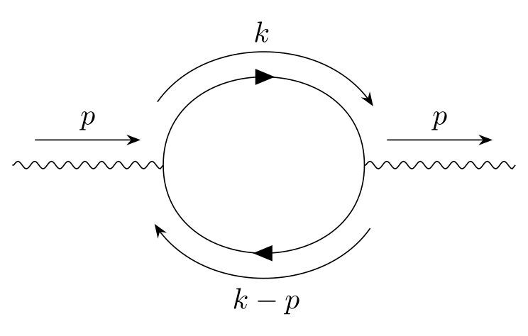
\usepackage{tikz} \usepackage[compat=1.1.0]{tikz-feynman}\begin{tikzpicture}
\begin{feynman}
\vertex (a) at (0, 0);
\vertex (b) at (1.8, 0);
\vertex (c) at (4.2, 0);
\vertex (d) at (6, 0);
\diagram* {
(a) -- [photon, momentum=\(p\)] (b)
-- [fermion, half left, momentum=\(k\)] (c)
-- [fermion, half left, momentum=\(k-p\)] (b),
(c) -- [photon, momentum=\(p\)] (d),
};
\end{feynman}
\end{tikzpicture}Full document
\documentclass[border=4pt]{standalone}
\usepackage{tikz}
\usepackage[compat=1.1.0]{tikz-feynman}
\begin{document}
\begin{tikzpicture}
  \begin{feynman}
    \vertex (a) at (0, 0);
    \vertex (b) at (1.8, 0);
    \vertex (c) at (4.2, 0);
    \vertex (d) at (6, 0);
    \diagram* {
      (a) -- [photon, momentum=\(p\)] (b)
          -- [fermion, half left, momentum=\(k\)] (c)
          -- [fermion, half left, momentum=\(k-p\)] (b),
      (c) -- [photon, momentum=\(p\)] (d),
    };
  \end{feynman}
\end{tikzpicture}
\end{document}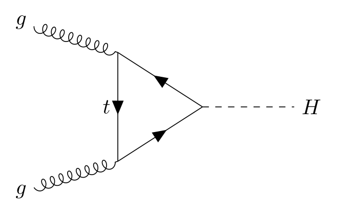
\usepackage{tikz} \usepackage[compat=1.1.0]{tikz-feynman}\begin{tikzpicture}
\begin{feynman}
\vertex (g1) at (0, 1.4) {\(g\)};
\vertex (g2) at (0, -1.4) {\(g\)};
\vertex (t1) at (1.6, 0.9);
\vertex (t2) at (1.6, -0.9);
\vertex (t3) at (3.0, 0);
\vertex (h) at (4.8, 0) {\(H\)};
\diagram* {
(g1) -- [gluon] (t1),
(g2) -- [gluon] (t2),
(t1) -- [fermion, edge label'=\(t\)] (t2)
-- [fermion] (t3) -- [fermion] (t1),
(t3) -- [scalar] (h),
};
\end{feynman}
\end{tikzpicture}Full document
\documentclass[border=4pt]{standalone}
\usepackage{tikz}
\usepackage[compat=1.1.0]{tikz-feynman}
\begin{document}
\begin{tikzpicture}
  \begin{feynman}
    \vertex (g1) at (0,  1.4) {\(g\)};
    \vertex (g2) at (0, -1.4) {\(g\)};
    \vertex (t1) at (1.6,  0.9);
    \vertex (t2) at (1.6, -0.9);
    \vertex (t3) at (3.0,  0);
    \vertex (h)  at (4.8,  0) {\(H\)};
    \diagram* {
      (g1) -- [gluon] (t1),
      (g2) -- [gluon] (t2),
      (t1) -- [fermion, edge label'=\(t\)] (t2)
           -- [fermion] (t3) -- [fermion] (t1),
      (t3) -- [scalar] (h),
    };
  \end{feynman}
\end{tikzpicture}
\end{document}Inline diagrams in equations (Feynman rules)
\feynmandiagram [inline=(d.base)] {…}; inside maths aligns the diagram so that the baseline of vertex d’s label sits on the baseline of the equation, and makes it a little more compact; baseline=(d.base) aligns without the extra styling. In a document you would write this inside equation or \[ … \]; with LuaLaTeX, because \feynmandiagram places the vertices itself.
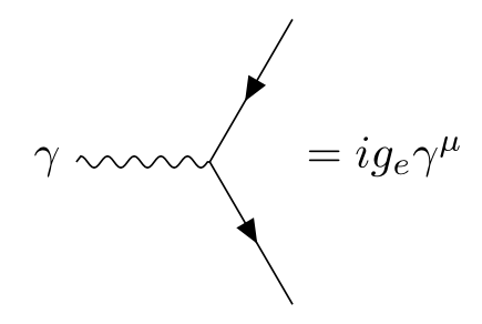
\usepackage{tikz} \usepackage[compat=1.1.0]{tikz-feynman}Compile with LuaLaTeX\begin{math}
\feynmandiagram [inline=(d.base), horizontal=d to b] {
a -- [fermion] b -- [fermion] c,
b -- [photon] d [particle=\(\gamma\)],
};
= i g_{e} \gamma^{\mu}
\end{math}Full document
\documentclass[border=4pt]{standalone}
\usepackage{tikz}
\usepackage[compat=1.1.0]{tikz-feynman}
\begin{document}
\begin{math}
  \feynmandiagram [inline=(d.base), horizontal=d to b] {
    a -- [fermion] b -- [fermion] c,
    b -- [photon] d [particle=\(\gamma\)],
  };
  = i g_{e} \gamma^{\mu}
\end{math}
\end{document}Customising: every fermion, every vertex, your own styles
\tikzfeynmanset changes the defaults for the whole document: \tikzfeynmanset{every vertex={dot}, every photon={blue}, every fermion={thick}}. More specific styles inherit from general ones (every scalar also applies to charged scalars). New styles are ordinary pgf keys, \tikzfeynmanset{myblob/.style={shape=circle, draw=blue, fill=red}}. Outside the feynman environment the keys need their full path, /tikzfeynman/fermion.
Alternatives: TikZ-FeynHand, feynMF and plain TikZ
- TikZ-FeynHand (1.1.0, 2019) is a modification of TikZ-Feynman that keeps only manual placement, so it never needs LuaLaTeX, and adds shorter keywords, extra vertex and propagator styles and a quick-start guide.
- feynMF/feynMP (1.08) is the older Metafont/MetaPost package that places vertices automatically; it needs an extra MetaPost run.
- For a single wavy or curly line in another drawing, plain TikZ decorations are enough:
\draw[decorate, decoration={snake}]or{coil, aspect=…}with\usetikzlibrary{decorations.pathmorphing}.
To try TikZ-Feynman code without installing anything, paste it into the LabCanvas TikZ editor, which compiles with TeX Live 2026 (the renderer behind these pictures, LuaLaTeX included).
Common errors and how to fix them
| LaTeX says (or you see) | Cause and fix |
|---|---|
| Package tikz-feynman Warning: LuaTeX is required if you wish to have vertices automatically placed. | You used \feynmandiagram or \diagram without positions under pdfLaTeX, and the vertices pile up. Compile with LuaLaTeX, or place the vertices with \vertex and connect them with \diagram*. |
| Package tikz Error: Giving up on this path. Did you forget a semicolon? | Every \vertex …;, every \diagram* {…}; and every \feynmandiagram {…}; must end with a semicolon. |
| Undefined control sequence. (at \vertex or \diagram) | \vertex and \diagram exist only inside \begin{feynman} … \end{feynman}, inside a tikzpicture. Also check that the package is loaded. |
| attempting to create edge between nodes that are not in the graph | LuaLaTeX, with vertices placed by \vertex and connected by \diagram. Use \diagram*, which connects existing vertices without running a layout. |
| Undefined control sequence. (at the closing }; of a diagram with particle= | The comma ended the key. Brace any label that contains a comma or square brackets: particle={\(\gamma, Z\)}, edge label={\(q, \bar q\)}. |
| A dot, blob or crossed dot does not appear | Give the vertex contents: \vertex [dot] (v) at (1,0) {};. Without {} it is a zero-size coordinate and the shape is not drawn. |
| layered layout, tree layout or horizontal=… has no effect | Under pdfLaTeX the graph drawing library is not loaded and these keys are ignored. Compile with LuaLaTeX. |
| A particle label or style given in \diagram* is missing | For a vertex declared with \vertex, give its options and label in the \vertex command; options written after its name inside \diagram* are ignored. |
Frequently asked questions
How do I draw a Feynman diagram in LaTeX?
Use TikZ-Feynman: \usepackage[compat=1.1.0]{tikz-feynman}, then place vertices with \vertex inside \begin{tikzpicture}\begin{feynman} … \end{feynman}\end{tikzpicture} and join them with \diagram* { (a) -- [fermion] (b) -- [photon] (c) };. With LuaLaTeX, \feynmandiagram can place the vertices for you.
Does TikZ-Feynman need LuaLaTeX?
Only for automatic placement (\feynmandiagram or \diagram without coordinates), which uses the Lua graph drawing algorithms of TikZ. Diagrams with manually placed vertices and \diagram* compile with pdfLaTeX, XeLaTeX and LuaLaTeX.
Is TikZ-Feynman still maintained? Does it work with current TeX Live?
The last release is 1.1.0 from February 2016 and the repository has seen no feature work since 2018, but it works: all diagrams on this page were compiled with TeX Live 2026. If you only need manual placement, TikZ-FeynHand (1.1.0, 2019) is a fork with the same syntax that drops the LuaLaTeX layouts.
How do I add momentum arrows?
Add momentum=\(p\) to the edge; momentum'= puts the arrow on the other side and reversed momentum= points it backwards. Style it with momentum={[arrow style=red]\(p\)}, since it does not take the edge’s colour.
How do I draw a loop in TikZ-Feynman?
Connect two vertices twice with curved edges: (b) -- [fermion, half left] (c) -- [fermion, half left] (b). For other shapes use quarter left, bend left, or out=90, in=90, looseness=1.5.
How do I use TikZ-Feynman on Overleaf?
TikZ-Feynman is installed on Overleaf. Manual placement works with the default pdfLaTeX; for \feynmandiagram set the compiler to LuaLaTeX in the project menu.
References
- TikZ-Feynman package on CTAN (v1.1.0, 2016-02-05)ctan.org
- TikZ-Feynman manual (PDF on CTAN)mirrors.ctan.org
- TikZ-Feynman manual, §2 Tutorialmirrors.ctan.org
- TikZ-Feynman manual, §2.4 When the algorithm isn’t enough (invisible edges, layouts, manual placement)mirrors.ctan.org
- TikZ-Feynman manual, §3.1 Commands & environmentsmirrors.ctan.org
- TikZ-Feynman manual, §3.2.2 Diagram keys (layouts)mirrors.ctan.org
- TikZ-Feynman manual, §3.2.3 Vertex keysmirrors.ctan.org
- TikZ-Feynman manual, §3.2.4 Edge keysmirrors.ctan.org
- TikZ-Feynman manual, §3.2.5 Momentum keys and §3.2.6 Modifier keysmirrors.ctan.org
- TikZ-Feynman manual, §4 Examplesmirrors.ctan.org
- J. Ellis, TikZ-Feynman: Feynman diagrams with TikZ, arXiv:1601.05437arxiv.org
- TikZ-Feynman project pagejpellis.me
- TikZ-Feynman repository (GitHub)github.com
- PGF/TikZ manual, §17.5.3 Advanced Placement Options (positioning)tikz.dev
- PGF/TikZ manual, §27 Introduction to Algorithmic Graph Drawingtikz.dev
- PGF/TikZ manual, §31 Layered Layoutstikz.dev
- PGF/TikZ manual, §32 Force-Based Methods (spring layout)tikz.dev
- TikZ-FeynHand package on CTAN (v1.1.0, 2019-08-19)ctan.org
The facts on this page were checked against these sources, and every picture is the code with it typeset with TeX Live 2026. Code on this page: CC0 1.0, copy it freely.
Try the code in your browserEvery snippet on this page opens in the free TikZ editor: it is typeset with TeX Live as you type, with errors pointed at their line.
Open the TikZ editor