TikZ physics diagrams: forces, springs, optics, waves and fields
Quick answer
arrows.meta for force arrows, angles and quotes for marked angles (\pic["$30^\circ$", draw] {angle=H--C--F};), decorations.pathmorphing for springs (decoration=coil), patterns for hatched walls and floors, and plot for waves. Draw each force from the point where it acts with a common style such as force/.style={-{Stealth[length=3mm]}, very thick}, and give the arrows lengths in proportion to the forces. The free-body diagram below is drawn to scale: F = 1.6, mg = 2, so N = mg − F sin 30° = 1.2 and, at constant velocity, f = F cos 30° ≈ 1.39.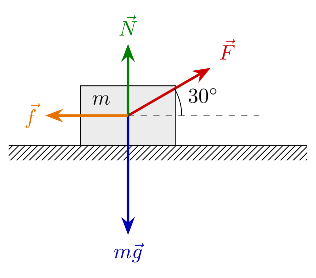
\usepackage{tikz} \usetikzlibrary{arrows.meta, angles, quotes, patterns}\begin{tikzpicture}[force/.style={-{Stealth[length=3mm]}, very thick}]
% ground and block
\fill[pattern=north east lines] (-2,-0.25) rectangle (3,0);
\draw (-2,0) -- (3,0);
\draw[fill=gray!15] (-0.8,0) rectangle (0.8,1);
\node at (-0.45,0.76) {$m$};
\coordinate (C) at (0,0.5);
% forces from the centre, to scale: F = 1.6, mg = 2,
% N = mg - F sin 30 = 1.2, f = F cos 30 = 1.39 (constant velocity)
\draw[dashed, gray] (C) -- (2.2,0.5) coordinate (H);
\draw[force, red!80!black] (C) -- ++(30:1.6) coordinate (F) node[above right] {$\vec F$};
\draw[force, blue!70!black] (C) -- ++(0,-2) node[below] {$m\vec g$};
\draw[force, green!50!black] (C) -- ++(0,1.2) node[above] {$\vec N$};
\draw[force, orange!90!black] (C) -- ++(-1.39,0) node[left] {$\vec f$};
\pic[draw, "$30^\circ$", angle radius=9mm, angle eccentricity=1.45] {angle=H--C--F};
\end{tikzpicture}Full document
\documentclass[border=4pt]{standalone}
\usepackage{tikz}
\usetikzlibrary{arrows.meta, angles, quotes, patterns}
\begin{document}
\begin{tikzpicture}[force/.style={-{Stealth[length=3mm]}, very thick}]
  % ground and block
  \fill[pattern=north east lines] (-2,-0.25) rectangle (3,0);
  \draw (-2,0) -- (3,0);
  \draw[fill=gray!15] (-0.8,0) rectangle (0.8,1);
  \node at (-0.45,0.76) {$m$};
  \coordinate (C) at (0,0.5);
  % forces from the centre, to scale: F = 1.6, mg = 2,
  % N = mg - F sin 30 = 1.2, f = F cos 30 = 1.39 (constant velocity)
  \draw[dashed, gray] (C) -- (2.2,0.5) coordinate (H);
  \draw[force, red!80!black]    (C) -- ++(30:1.6)  coordinate (F) node[above right] {$\vec F$};
  \draw[force, blue!70!black]   (C) -- ++(0,-2)    node[below] {$m\vec g$};
  \draw[force, green!50!black]  (C) -- ++(0,1.2)   node[above] {$\vec N$};
  \draw[force, orange!90!black] (C) -- ++(-1.39,0) node[left] {$\vec f$};
  \pic[draw, "$30^\circ$", angle radius=9mm, angle eccentricity=1.45] {angle=H--C--F};
\end{tikzpicture}
\end{document}Contents
Free-body diagrams: force vectors and angles
The diagram at the top has three ingredients. A force style keeps every arrow the same thickness with a clearly visible tip; each force starts at the centre (C) and is given relative to it, (C) -- ++(30:1.6) in polar form for the slanted pull, so that changing one number moves one arrow. The labels are nodes at the arrow ends with above right, below or left, so they never sit on a line, and \vec F or bold \mathbf F marks them as vectors.
The angle comes from the angles library: \pic[draw, "$30^\circ$"] {angle=H--C--F} draws the arc at C from the ray towards H counter-clockwise to the ray towards F, so the order of the three points matters. angle radius (initially 5mm) sets the arc’s size and angle eccentricity (initially 0.6) how far out the label sits, as a fraction of the radius; a value above 1 puts the label outside the arc. The quoted label needs the quotes library as well. The points must be named coordinates, which is why the force is written with coordinate (F) at its tip. For a right angle there is \pic[draw] {right angle=A--B--C}.
Strictly, a free-body diagram shows the body alone, often as a dot, with every force acting on it; the block and ground are drawn here for orientation. If the forces are meant to balance, check it: here the vertical components give N + F sin 30° = mg, 1.2 + 0.8 = 2, and the horizontal ones F cos 30° = f.
Inclined plane: resolving the weight
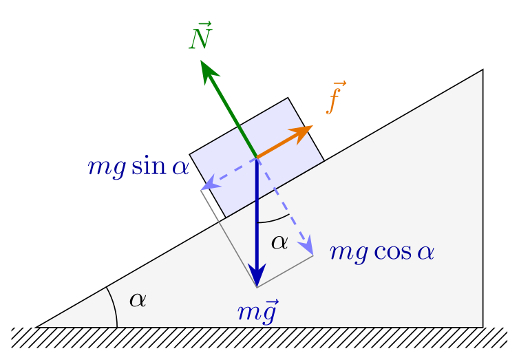
On a slope everything except gravity is aligned with the surface, so draw the block and its forces in a scope rotated by the slope angle: inside \begin{scope}[rotate=30], x runs along the slope and y perpendicular to it. The one exception is the weight, which still points straight down: in the rotated frame that is the direction −90° − 30° = −120°, hence (C) -- ++(-120:1.6). Its components are then axis-aligned in the scope: mg sin α = 0.8 down the slope and mg cos α ≈ 1.39 into it, drawn dashed with the thin lines that complete the parallelogram.
A block at rest has N = mg cos α and a static friction force f = mg sin α up the slope, which is how the arrows are sized. The angle between the weight and the perpendicular component equals the slope angle α, which the second angle pic shows; the slope itself is a triangle whose top corner is at height 5.5 tan 30°.
\usepackage{tikz} \usetikzlibrary{arrows.meta, angles, quotes, patterns}\begin{tikzpicture}[force/.style={-{Stealth[length=3mm]}, very thick},
part/.style={-{Stealth[length=2.5mm]}, thick, dashed}]
% the incline: 30 degrees
\coordinate (O) at (0,0);
\coordinate (R) at (5.5,0);
\coordinate (T) at (5.5,{5.5*tan(30)});
\fill[pattern=north east lines] (-0.3,-0.25) rectangle (5.8,0);
\draw[fill=gray!8] (O) -- (R) -- (T) -- cycle;
\pic[draw, "$\alpha$", angle radius=10mm, angle eccentricity=1.3] {angle=R--O--T};
% everything on the slope in a rotated scope: x along the slope, y perpendicular
\begin{scope}[rotate=30]
\draw[fill=blue!10] (2.7,0) rectangle (4.1,0.9);
\coordinate (C) at (3.4,0.45);
% weight straight down = -120 degrees in this frame; mg = 1.6
\draw[force, blue!70!black] (C) -- ++(-120:1.6) coordinate (W) node[below] {$m\vec g$};
\draw[part, blue!50] (C) -- ++(-0.8,0) coordinate (Wt) node[above left, blue!60!black] {$mg\sin\alpha$};
\draw[part, blue!50] (C) -- ++(0,-1.39) coordinate (Wn);
\node[blue!60!black, right=2pt] at (Wn) {$mg\cos\alpha$};
\draw[gray, thin] (Wt) -- (W) -- (Wn);
\draw[force, green!50!black] (C) -- ++(0,1.39) node[above] {$\vec N$};
\draw[force, orange!90!black] (C) -- ++(0.8,0) node[above right] {$\vec f$};
\pic[draw, "$\alpha$", angle radius=8mm, angle eccentricity=1.35] {angle=W--C--Wn};
\end{scope}
\end{tikzpicture}Full document
\documentclass[border=4pt]{standalone}
\usepackage{tikz}
\usetikzlibrary{arrows.meta, angles, quotes, patterns}
\begin{document}
\begin{tikzpicture}[force/.style={-{Stealth[length=3mm]}, very thick},
                    part/.style={-{Stealth[length=2.5mm]}, thick, dashed}]
  % the incline: 30 degrees
  \coordinate (O) at (0,0);
  \coordinate (R) at (5.5,0);
  \coordinate (T) at (5.5,{5.5*tan(30)});
  \fill[pattern=north east lines] (-0.3,-0.25) rectangle (5.8,0);
  \draw[fill=gray!8] (O) -- (R) -- (T) -- cycle;
  \pic[draw, "$\alpha$", angle radius=10mm, angle eccentricity=1.3] {angle=R--O--T};
  % everything on the slope in a rotated scope: x along the slope, y perpendicular
  \begin{scope}[rotate=30]
    \draw[fill=blue!10] (2.7,0) rectangle (4.1,0.9);
    \coordinate (C) at (3.4,0.45);
    % weight straight down = -120 degrees in this frame; mg = 1.6
    \draw[force, blue!70!black] (C) -- ++(-120:1.6) coordinate (W) node[below] {$m\vec g$};
    \draw[part, blue!50] (C) -- ++(-0.8,0) coordinate (Wt) node[above left, blue!60!black] {$mg\sin\alpha$};
    \draw[part, blue!50] (C) -- ++(0,-1.39) coordinate (Wn);
    \node[blue!60!black, right=2pt] at (Wn) {$mg\cos\alpha$};
    \draw[gray, thin] (Wt) -- (W) -- (Wn);
    \draw[force, green!50!black]  (C) -- ++(0,1.39) node[above] {$\vec N$};
    \draw[force, orange!90!black] (C) -- ++(0.8,0)  node[above right] {$\vec f$};
    \pic[draw, "$\alpha$", angle radius=8mm, angle eccentricity=1.35] {angle=W--C--Wn};
  \end{scope}
\end{tikzpicture}
\end{document}Springs: the coil decoration
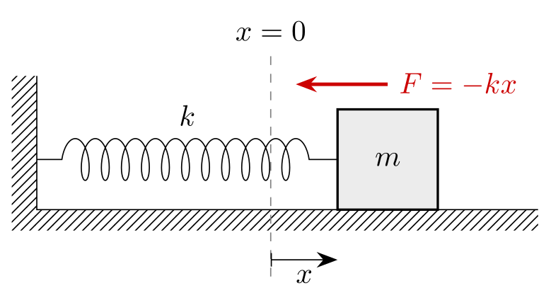
A spring is a straight line drawn with a decoration from \usetikzlibrary{decorations.pathmorphing}: decorate, decoration={coil, …}. The coil is a helix seen from the side: amplitude (initially 2.5pt) is its radius, segment length (initially 10pt) the distance between two turns, and aspect (initially 0.5) the viewing direction, 0 giving a plain sine wave. pre length and post length keep straight pieces at both ends, where the spring is fixed. Defining it once as a spring style makes every spring in a document match. zigzag instead of coil gives the flat textbook spring.
The picture shows Hooke’s law: with the block a distance x to the right of its equilibrium position, the spring pulls it back with F = −kx, towards x = 0. The wall and floor are hatched with the patterns library: \fill[pattern=north east lines] on a thin rectangle, with the surface drawn as a solid line on top.
\usepackage{tikz} \usetikzlibrary{arrows.meta, decorations.pathmorphing, patterns}\begin{tikzpicture}[>={Stealth[length=2.5mm]},
spring/.style={decorate, decoration={coil, aspect=0.4, segment length=2.4mm,
amplitude=2.5mm, pre length=3mm, post length=3mm}}]
% wall and floor
\fill[pattern=north east lines] (-0.3,-0.25) rectangle (0,1.6);
\fill[pattern=north east lines] (0,-0.25) rectangle (6,0);
\draw (0,1.6) -- (0,0) -- (6,0);
% equilibrium position of the block's left face, and the displaced block
\draw[dashed, gray] (2.8,-0.8) -- (2.8,1.9) node[above, black] {$x=0$};
\draw[thick, fill=gray!15] (3.6,0) rectangle (4.8,1.2) node[midway] {$m$};
\draw[spring] (0,0.6) -- node[above=8pt] {$k$} (3.6,0.6);
\draw[|->] (2.8,-0.6) -- node[below] {$x$} (3.6,-0.6);
% restoring force of the spring on the block: towards x = 0
\draw[->, very thick, red!80!black] (4.2,1.5) node[right] {$F = -kx$} -- ++(-1.1,0);
\end{tikzpicture}Full document
\documentclass[border=4pt]{standalone}
\usepackage{tikz}
\usetikzlibrary{arrows.meta, decorations.pathmorphing, patterns}
\begin{document}
\begin{tikzpicture}[>={Stealth[length=2.5mm]},
    spring/.style={decorate, decoration={coil, aspect=0.4, segment length=2.4mm,
                   amplitude=2.5mm, pre length=3mm, post length=3mm}}]
  % wall and floor
  \fill[pattern=north east lines] (-0.3,-0.25) rectangle (0,1.6);
  \fill[pattern=north east lines] (0,-0.25) rectangle (6,0);
  \draw (0,1.6) -- (0,0) -- (6,0);
  % equilibrium position of the block's left face, and the displaced block
  \draw[dashed, gray] (2.8,-0.8) -- (2.8,1.9) node[above, black] {$x=0$};
  \draw[thick, fill=gray!15] (3.6,0) rectangle (4.8,1.2) node[midway] {$m$};
  \draw[spring] (0,0.6) -- node[above=8pt] {$k$} (3.6,0.6);
  \draw[|->] (2.8,-0.6) -- node[below] {$x$} (3.6,-0.6);
  % restoring force of the spring on the block: towards x = 0
  \draw[->, very thick, red!80!black] (4.2,1.5) node[right] {$F = -kx$} -- ++(-1.1,0);
\end{tikzpicture}
\end{document}Pendulum: angle, equilibrium line and forces
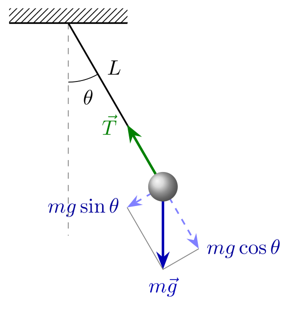
Put the pivot at the origin and the bob in polar coordinates, ({-90+\Th}:\Len): angle −90° is straight down, so the string makes the angle \Th with the dashed vertical, which the angle pic marks between (V) on the vertical and (B) at the bob. All force directions follow from the same angle, so changing \Th redraws the whole picture correctly: the tension points back along the string, ({90+\Th}:…), and the weight splits into mg cos θ along the string and mg sin θ perpendicular to it, towards the equilibrium position. That component is the restoring force; for small angles it gives the period 2π√(L/g). The arrows are drawn at a turning point, where the bob is momentarily at rest and the tension equals mg cos θ. The bob is shaded last, with ball color, so that it covers the ends of the arrows.
\usepackage{tikz} \usetikzlibrary{arrows.meta, angles, quotes, patterns}\begin{tikzpicture}[force/.style={-{Stealth[length=3mm]}, very thick},
part/.style={-{Stealth[length=2.5mm]}, thick, dashed}]
\def\Len{3.2} % length of the string
\def\Th{30} % angle from the vertical (degrees)
% support and the dashed equilibrium line
\fill[pattern=north east lines] (-1,0) rectangle (1,0.25);
\draw[thick] (-1,0) -- (1,0);
\coordinate (O) at (0,0);
\draw[dashed, gray] (O) -- (0,-\Len-0.4) coordinate (V);
% string and bob
\draw[thick] (O) -- node[pos=0.35, above right=-1pt] {$L$} ({-90+\Th}:\Len) coordinate (B);
\pic[draw, "$\theta$", angle radius=10mm, angle eccentricity=1.3] {angle=V--O--B};
% forces on the bob, mg = 1.4; at the turning point T = mg cos(theta)
\draw[force, blue!70!black] (B) -- ++(0,-1.4) coordinate (W) node[below] {$m\vec g$};
\draw[force, green!50!black] (B) -- ++({90+\Th}:{1.4*cos(\Th)}) node[left=1pt] {$\vec T$};
\draw[part, blue!50] (B) -- ++({-180+\Th}:{1.4*sin(\Th)}) coordinate (Wt)
node[left, blue!60!black] {$mg\sin\theta$};
\draw[part, blue!50] (B) -- ++({-90+\Th}:{1.4*cos(\Th)}) coordinate (Wr)
node[right, blue!60!black] {$mg\cos\theta$};
\draw[gray, thin] (Wt) -- (W) -- (Wr);
\shade[ball color=gray!40] (B) circle[radius=2.5mm];
\end{tikzpicture}Full document
\documentclass[border=4pt]{standalone}
\usepackage{tikz}
\usetikzlibrary{arrows.meta, angles, quotes, patterns}
\begin{document}
\begin{tikzpicture}[force/.style={-{Stealth[length=3mm]}, very thick},
                    part/.style={-{Stealth[length=2.5mm]}, thick, dashed}]
  \def\Len{3.2}   % length of the string
  \def\Th{30}   % angle from the vertical (degrees)
  % support and the dashed equilibrium line
  \fill[pattern=north east lines] (-1,0) rectangle (1,0.25);
  \draw[thick] (-1,0) -- (1,0);
  \coordinate (O) at (0,0);
  \draw[dashed, gray] (O) -- (0,-\Len-0.4) coordinate (V);
  % string and bob
  \draw[thick] (O) -- node[pos=0.35, above right=-1pt] {$L$} ({-90+\Th}:\Len) coordinate (B);
  \pic[draw, "$\theta$", angle radius=10mm, angle eccentricity=1.3] {angle=V--O--B};
  % forces on the bob, mg = 1.4; at the turning point T = mg cos(theta)
  \draw[force, blue!70!black]  (B) -- ++(0,-1.4) coordinate (W) node[below] {$m\vec g$};
  \draw[force, green!50!black] (B) -- ++({90+\Th}:{1.4*cos(\Th)}) node[left=1pt] {$\vec T$};
  \draw[part, blue!50] (B) -- ++({-180+\Th}:{1.4*sin(\Th)}) coordinate (Wt)
    node[left, blue!60!black] {$mg\sin\theta$};
  \draw[part, blue!50] (B) -- ++({-90+\Th}:{1.4*cos(\Th)}) coordinate (Wr)
    node[right, blue!60!black] {$mg\cos\theta$};
  \draw[gray, thin] (Wt) -- (W) -- (Wr);
  \shade[ball color=gray!40] (B) circle[radius=2.5mm];
\end{tikzpicture}
\end{document}Ray diagrams: a converging lens
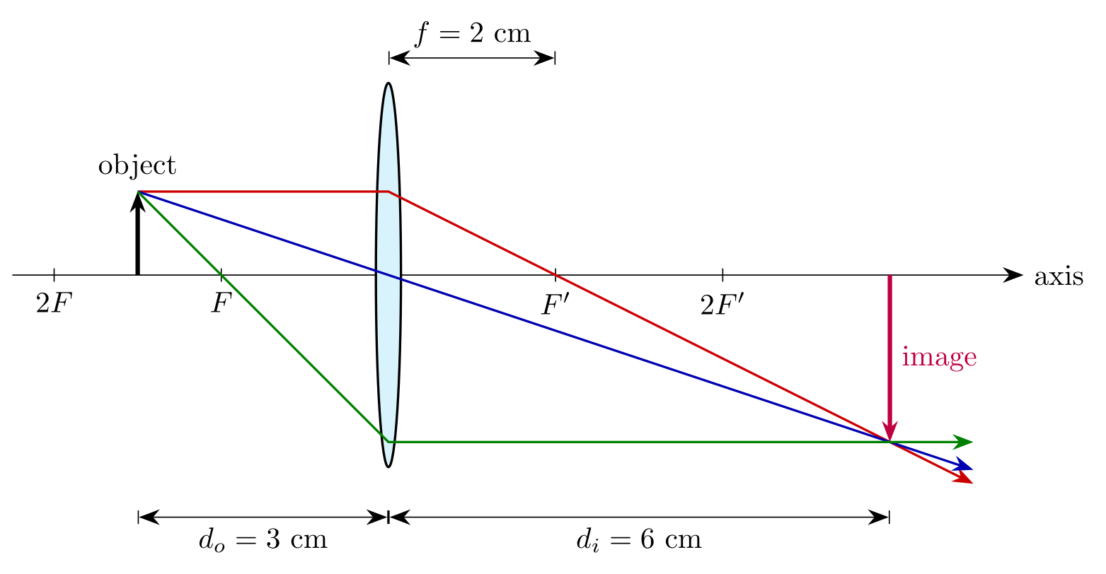
For a thin lens of focal length f, the object distance do and image distance di satisfy 1/do + 1/di = 1/f, and the magnification is m = −di/do. The first diagram uses f = 2 cm and an object 1 cm tall at do = 3 cm: 1/di = 1/2 − 1/3 = 1/6, so the image is at di = 6 cm, real, inverted and twice as large (m = −2), with its tip at (6, −2). With 1 cm per unit, the three principal rays are exact straight lines:
- parallel to the axis, then through the far focal point F′ = (2, 0): from (0, 1) the slope is −1/2, which reaches (6, −2);
- through the centre of the lens, undeviated: slope −1/3 from (−3, 1), also reaching (6, −2);
- through the near focal point F = (−2, 0), which it meets at slope −1, so it reaches the lens at (0, −2) and leaves parallel to the axis.
The thin-lens model bends every ray once, in the plane of the lens, so each ray is a path with a corner at x = 0. The second diagram puts the object inside the focal length (do = 1 cm): 1/di = 1/2 − 1 = −1/2, so di = −2 cm, a virtual, upright image twice as large (m = +2), as in a magnifying glass. The refracted rays diverge, and their backward extensions, drawn dashed, meet at (−2, 2), where the image is drawn dashed as well.
For optical setups with lasers, mirrors and detectors rather than textbook ray diagrams, the LabCanvas Optics app lays out components on a virtual table and traces the rays for you, without code.
\usepackage{tikz} \usetikzlibrary{arrows.meta}\begin{tikzpicture}[>={Stealth[length=2.5mm]}, ray/.style={thick, ->}]
% f = 2 cm, object 1 cm tall at d_o = 3 cm:
% 1/d_i = 1/2 - 1/3 = 1/6, so d_i = 6 cm and m = -d_i/d_o = -2
\draw[->] (-4.5,0) -- (7.6,0) node[right] {axis};
\draw[thick, fill=cyan!15] (0,0) ellipse[x radius=0.15, y radius=2.3];
\foreach \x/\n in {-4/2F, -2/F, 2/F', 4/2F'}
\draw (\x,0.08) -- (\x,-0.08) node[below] {$\n$};
% object and (real, inverted) image
\draw[->, line width=1.5pt] (-3,0) -- (-3,1) node[above] {object};
\draw[->, line width=1.5pt, purple] (6,0) -- node[right] {image} (6,-2);
% 1: parallel to the axis, then through F'
\draw[ray, red!80!black] (-3,1) -- (0,1) -- (7,-2.5);
% 2: through the centre of the lens, undeviated
\draw[ray, blue!70!black] (-3,1) -- (7,{-7/3});
% 3: through F, then parallel to the axis
\draw[ray, green!50!black] (-3,1) -- (0,-2) -- (7,-2);
% distances
\draw[|<->|] (-3,-2.9) -- node[below] {$d_o = 3$ cm} (0,-2.9);
\draw[|<->|] (0,-2.9) -- node[below] {$d_i = 6$ cm} (6,-2.9);
\draw[|<->|] (0,2.6) -- node[above] {$f = 2$ cm} (2,2.6);
\end{tikzpicture}Full document
\documentclass[border=4pt]{standalone}
\usepackage{tikz}
\usetikzlibrary{arrows.meta}
\begin{document}
\begin{tikzpicture}[>={Stealth[length=2.5mm]}, ray/.style={thick, ->}]
  % f = 2 cm, object 1 cm tall at d_o = 3 cm:
  % 1/d_i = 1/2 - 1/3 = 1/6, so d_i = 6 cm and m = -d_i/d_o = -2
  \draw[->] (-4.5,0) -- (7.6,0) node[right] {axis};
  \draw[thick, fill=cyan!15] (0,0) ellipse[x radius=0.15, y radius=2.3];
  \foreach \x/\n in {-4/2F, -2/F, 2/F', 4/2F'}
    \draw (\x,0.08) -- (\x,-0.08) node[below] {$\n$};
  % object and (real, inverted) image
  \draw[->, line width=1.5pt] (-3,0) -- (-3,1) node[above] {object};
  \draw[->, line width=1.5pt, purple] (6,0) -- node[right] {image} (6,-2);
  % 1: parallel to the axis, then through F'
  \draw[ray, red!80!black]   (-3,1) -- (0,1) -- (7,-2.5);
  % 2: through the centre of the lens, undeviated
  \draw[ray, blue!70!black]  (-3,1) -- (7,{-7/3});
  % 3: through F, then parallel to the axis
  \draw[ray, green!50!black] (-3,1) -- (0,-2) -- (7,-2);
  % distances
  \draw[|<->|] (-3,-2.9) -- node[below] {$d_o = 3$ cm} (0,-2.9);
  \draw[|<->|] (0,-2.9) -- node[below] {$d_i = 6$ cm} (6,-2.9);
  \draw[|<->|] (0,2.6) -- node[above] {$f = 2$ cm} (2,2.6);
\end{tikzpicture}
\end{document}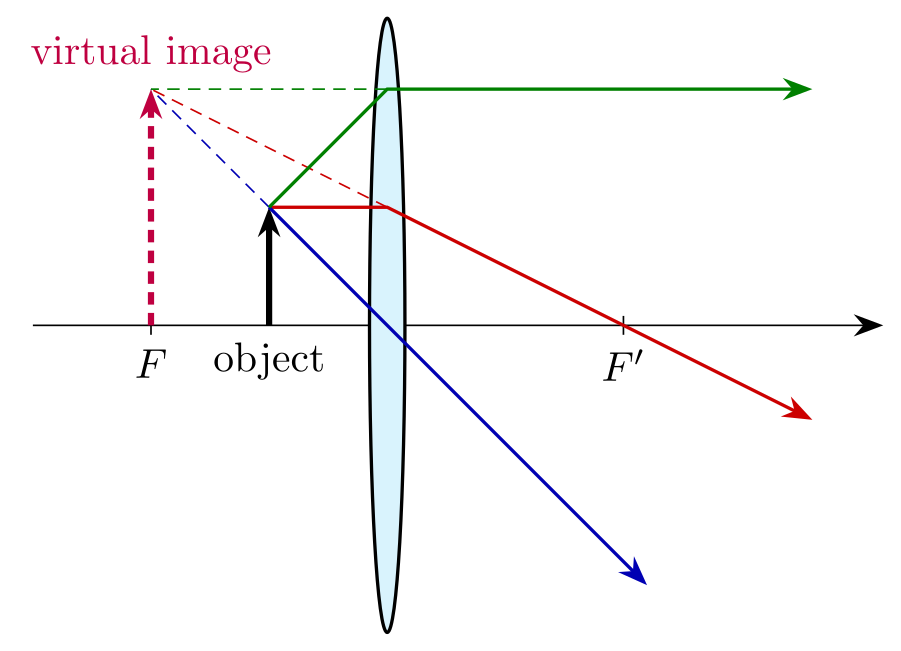
\usepackage{tikz} \usetikzlibrary{arrows.meta}\begin{tikzpicture}[>={Stealth[length=2.5mm]}, ray/.style={thick, ->},
back/.style={thin, densely dashed}]
% object inside the focal length: f = 2 cm, d_o = 1 cm
% 1/d_i = 1/2 - 1/1 = -1/2, so d_i = -2 cm (virtual), m = +2 (upright)
\draw[->] (-3,0) -- (4.2,0);
\draw[thick, fill=cyan!15] (0,0) ellipse[x radius=0.15, y radius=2.6];
\foreach \x/\n in {-2/F, 2/F'}
\draw (\x,0.08) -- (\x,-0.08) node[below] {$\n$};
\draw[->, line width=1.5pt] (-1,0) node[below] {object} -- (-1,1);
% the rays that leave the lens, and their backward extensions (dashed)
\draw[ray, red!80!black] (-1,1) -- (0,1) -- (3.6,-0.8);
\draw[back, red!80!black] (0,1) -- (-2,2);
\draw[ray, blue!70!black] (-1,1) -- (2.2,-2.2);
\draw[back, blue!70!black] (-1,1) -- (-2,2);
\draw[ray, green!50!black] (-1,1) -- (0,2) -- (3.6,2);
\draw[back, green!50!black] (0,2) -- (-2,2);
% the virtual image: where the extensions meet
\draw[->, line width=1.5pt, purple, densely dashed] (-2,0) -- (-2,2)
node[above] {virtual image};
\end{tikzpicture}Full document
\documentclass[border=4pt]{standalone}
\usepackage{tikz}
\usetikzlibrary{arrows.meta}
\begin{document}
\begin{tikzpicture}[>={Stealth[length=2.5mm]}, ray/.style={thick, ->},
                    back/.style={thin, densely dashed}]
  % object inside the focal length: f = 2 cm, d_o = 1 cm
  % 1/d_i = 1/2 - 1/1 = -1/2, so d_i = -2 cm (virtual), m = +2 (upright)
  \draw[->] (-3,0) -- (4.2,0);
  \draw[thick, fill=cyan!15] (0,0) ellipse[x radius=0.15, y radius=2.6];
  \foreach \x/\n in {-2/F, 2/F'}
    \draw (\x,0.08) -- (\x,-0.08) node[below] {$\n$};
  \draw[->, line width=1.5pt] (-1,0) node[below] {object} -- (-1,1);
  % the rays that leave the lens, and their backward extensions (dashed)
  \draw[ray, red!80!black]   (-1,1) -- (0,1) -- (3.6,-0.8);
  \draw[back, red!80!black]  (0,1) -- (-2,2);
  \draw[ray, blue!70!black]  (-1,1) -- (2.2,-2.2);
  \draw[back, blue!70!black] (-1,1) -- (-2,2);
  \draw[ray, green!50!black] (-1,1) -- (0,2) -- (3.6,2);
  \draw[back, green!50!black] (0,2) -- (-2,2);
  % the virtual image: where the extensions meet
  \draw[->, line width=1.5pt, purple, densely dashed] (-2,0) -- (-2,2)
    node[above] {virtual image};
\end{tikzpicture}
\end{document}Waves: plotting a sine
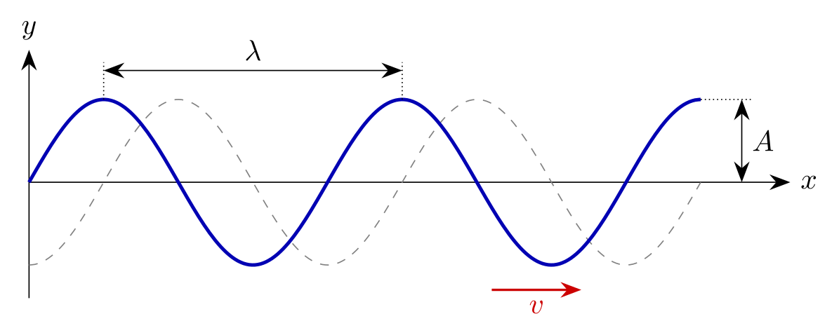
\draw plot[domain=0:9, samples=120, smooth] (\x, {sin(2*pi*\x/4 r)}); draws y = A sin(2πx/λ) with A = 1 and λ = 4. Two details matter. PGF’s trigonometric functions work in degrees, so an argument in radians needs the r operator (or the key trig format=rad); without it the argument only reaches 14° and the wave comes out as an almost flat line. And the default of 25 samples over the default domain −5 to 5 is too coarse for several periods, so set both. Crests are at x = 1, 5, 9, which is where the wavelength and amplitude are marked. The dashed curve is the same function of x − 1, the wave a quarter period later, moving in the direction of v.
x=0.9cm on the picture squeezes it horizontally without touching the code. For several waves, axes with ticks or a legend, pgfplots is easier (\addplot[domain=0:9, samples=120] {sin(deg(2*pi*x/4))}; inside an axis).
\usepackage{tikz} \usetikzlibrary{arrows.meta}\begin{tikzpicture}[>={Stealth[length=2.5mm]}, x=0.9cm]
% y = A sin(2 pi x / lambda) with A = 1, lambda = 4: the argument is in radians, hence "r"
\draw[->] (0,0) -- (10.2,0) node[right] {$x$};
\draw[->] (0,-1.4) -- (0,1.6) node[above] {$y$};
\draw[dashed, gray] plot[domain=0:9, samples=120, smooth] (\x, {sin(2*pi*(\x-1)/4 r)});
\draw[very thick, blue!70!black] plot[domain=0:9, samples=120, smooth] (\x, {sin(2*pi*\x/4 r)});
% wavelength between two crests, amplitude at the third crest
\draw[densely dotted] (1,1) -- (1,1.45) (5,1) -- (5,1.45);
\draw[<->] (1,1.35) -- node[above] {$\lambda$} (5,1.35);
\draw[densely dotted] (9,1) -- (9.7,1);
\draw[<->] (9.55,0) -- node[right] {$A$} (9.55,1);
% the dashed curve is the same wave a moment later
\draw[->, thick, red!80!black] (6.2,-1.3) -- node[below] {$v$} (7.4,-1.3);
\end{tikzpicture}Full document
\documentclass[border=4pt]{standalone}
\usepackage{tikz}
\usetikzlibrary{arrows.meta}
\begin{document}
\begin{tikzpicture}[>={Stealth[length=2.5mm]}, x=0.9cm]
  % y = A sin(2 pi x / lambda) with A = 1, lambda = 4: the argument is in radians, hence "r"
  \draw[->] (0,0) -- (10.2,0) node[right] {$x$};
  \draw[->] (0,-1.4) -- (0,1.6) node[above] {$y$};
  \draw[dashed, gray] plot[domain=0:9, samples=120, smooth] (\x, {sin(2*pi*(\x-1)/4 r)});
  \draw[very thick, blue!70!black] plot[domain=0:9, samples=120, smooth] (\x, {sin(2*pi*\x/4 r)});
  % wavelength between two crests, amplitude at the third crest
  \draw[densely dotted] (1,1) -- (1,1.45)  (5,1) -- (5,1.45);
  \draw[<->] (1,1.35) -- node[above] {$\lambda$} (5,1.35);
  \draw[densely dotted] (9,1) -- (9.7,1);
  \draw[<->] (9.55,0) -- node[right] {$A$} (9.55,1);
  % the dashed curve is the same wave a moment later
  \draw[->, thick, red!80!black] (6.2,-1.3) -- node[below] {$v$} (7.4,-1.3);
\end{tikzpicture}
\end{document}Energy-level diagrams
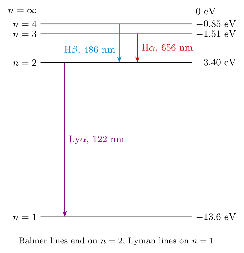
An energy-level diagram is a set of horizontal lines at heights proportional to energy, and a \foreach over level/energy pairs draws them with their labels. The hydrogen diagram is to scale: y=0.5cm makes one unit of y half a centimetre, so the levels can be written directly in electronvolts, En = −13.6 eV/n2: −13.6, −3.40, −1.51 and −0.85 eV, crowding towards the ionisation limit at 0. Transitions are vertical arrows from the upper to the lower level for emission (reverse them for absorption). The photon energy is the difference of the levels, and the wavelength hc/ΔE: 3 → 2 is 1.89 eV or 656 nm (Hα, red), 4 → 2 is 2.55 eV or 486 nm (Hβ), and 2 → 1 is 10.2 eV or 122 nm (Lyman α, ultraviolet). For molecular orbital diagrams, see the molecular orbital diagram generator.
\usepackage{tikz} \usetikzlibrary{arrows.meta}\begin{tikzpicture}[y=0.5cm, >={Stealth[length=2mm]}, font=\small]
% hydrogen, E_n = -13.6 eV / n^2, drawn to scale (0.5 cm per eV)
\foreach \n/\E in {1/-13.6, 2/-3.40, 3/-1.51, 4/-0.85} {
\draw[thick] (0,\E) -- (5,\E);
\node[left] at (0,\E) {$n=\n$};
\node[right] at (5,\E) {$\E$ eV};
}
\draw[dashed] (0,0) -- (5,0);
\node[left] at (0,0) {$n=\infty$};
\node[right] at (5,0) {$0$ eV};
% emission lines: Lyman alpha (ultraviolet), Balmer H-alpha and H-beta (visible)
\draw[->, thick, violet] (0.8,-3.40) -- node[right] {Ly$\alpha$, 122 nm} (0.8,-13.6);
\draw[->, thick, red!85!black] (3.2,-1.51) -- (3.2,-3.40) node[pos=0.5, right] {H$\alpha$, 656 nm};
\draw[->, thick, cyan!70!blue] (2.6,-0.85) -- (2.6,-3.40) node[pos=0.68, left] {H$\beta$, 486 nm};
\node[font=\footnotesize] at (2.5,-15.2) {Balmer lines end on $n=2$, Lyman lines on $n=1$};
\end{tikzpicture}Full document
\documentclass[border=4pt]{standalone}
\usepackage{tikz}
\usetikzlibrary{arrows.meta}
\begin{document}
\begin{tikzpicture}[y=0.5cm, >={Stealth[length=2mm]}, font=\small]
  % hydrogen, E_n = -13.6 eV / n^2, drawn to scale (0.5 cm per eV)
  \foreach \n/\E in {1/-13.6, 2/-3.40, 3/-1.51, 4/-0.85} {
    \draw[thick] (0,\E) -- (5,\E);
    \node[left]  at (0,\E) {$n=\n$};
    \node[right] at (5,\E) {$\E$ eV};
  }
  \draw[dashed] (0,0) -- (5,0);
  \node[left] at (0,0) {$n=\infty$};
  \node[right] at (5,0) {$0$ eV};
  % emission lines: Lyman alpha (ultraviolet), Balmer H-alpha and H-beta (visible)
  \draw[->, thick, violet]       (0.8,-3.40) -- node[right] {Ly$\alpha$, 122 nm} (0.8,-13.6);
  \draw[->, thick, red!85!black] (3.2,-1.51) -- (3.2,-3.40) node[pos=0.5, right] {H$\alpha$, 656 nm};
  \draw[->, thick, cyan!70!blue] (2.6,-0.85) -- (2.6,-3.40) node[pos=0.68, left] {H$\beta$, 486 nm};
  \node[font=\footnotesize] at (2.5,-15.2) {Balmer lines end on $n=2$, Lyman lines on $n=1$};
\end{tikzpicture}
\end{document}Vector fields and field lines
A field drawn as arrows on a grid is two nested \foreach loops and a little pgfmath. The dipole below has +q at (−1, 0) and −q at (1, 0); at each grid point the field is proportional to (r − r1)/|r − r1|³ − (r − r2)/|r − r2|³, atan2(Ey, Ex) (note the order: y first) gives its direction, and the arrow is drawn centred on the point with a fixed length. Fixed-length arrows show the direction everywhere; arrows scaled by the field strength would be invisible in most places and huge near the charges. Points closer than 0.4 to a charge are skipped, which avoids dividing by zero at the charges themselves. Put the loop variables in parentheses, (\y)^2: with \y = −2, \y^2 becomes -2^2, which pgfmath reads as −(2²) = −4.
For a field given by a formula on a plot with axes, the pgfplots quiver plot type does the same with quiver={u=…, v=…}. Smooth field lines need the field integrated along the lines, which TikZ does not do; compute them elsewhere and plot the points, or sketch them with to[out=…, in=…].
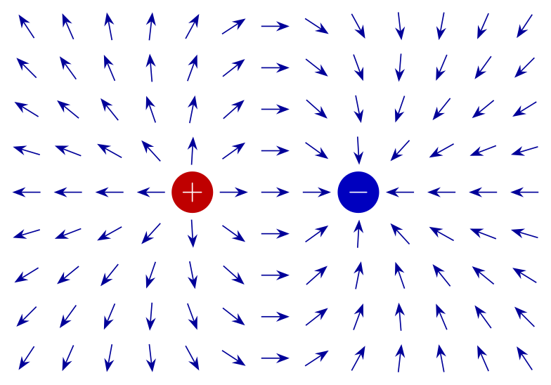
\usepackage{tikz} \usetikzlibrary{arrows.meta}\begin{tikzpicture}[>={Stealth[length=1.6mm]}]
% field direction of +q at (-1,0) and -q at (1,0) on a grid:
% E is proportional to (r - r1)/|r - r1|^3 - (r - r2)/|r - r2|^3
\foreach \x in {-3,-2.5,...,3} {
\foreach \y in {-2,-1.5,...,2} {
\pgfmathsetmacro\ra{sqrt((\x+1)^2 + (\y)^2)} % distance to +q
\pgfmathsetmacro\rb{sqrt((\x-1)^2 + (\y)^2)} % distance to -q
\pgfmathtruncatemacro\far{and(\ra > 0.4, \rb > 0.4)}
\ifnum\far=1
\pgfmathsetmacro\Ex{(\x+1)/\ra^3 - (\x-1)/\rb^3}
\pgfmathsetmacro\Ey{(\y)/\ra^3 - (\y)/\rb^3}
\pgfmathsetmacro\ang{atan2(\Ey, \Ex)}
\draw[->, blue!60!black] (\x,\y) ++(\ang:-0.17) -- ++(\ang:0.34);
\fi
}
}
\node[circle, fill=red!75!black, text=white, inner sep=1pt, minimum size=5mm] at (-1,0) {$+$};
\node[circle, fill=blue!75!black, text=white, inner sep=1pt, minimum size=5mm] at (1,0) {$-$};
\end{tikzpicture}Full document
\documentclass[border=4pt]{standalone}
\usepackage{tikz}
\usetikzlibrary{arrows.meta}
\begin{document}
\begin{tikzpicture}[>={Stealth[length=1.6mm]}]
  % field direction of +q at (-1,0) and -q at (1,0) on a grid:
  % E is proportional to (r - r1)/|r - r1|^3 - (r - r2)/|r - r2|^3
  \foreach \x in {-3,-2.5,...,3} {
    \foreach \y in {-2,-1.5,...,2} {
      \pgfmathsetmacro\ra{sqrt((\x+1)^2 + (\y)^2)}   % distance to +q
      \pgfmathsetmacro\rb{sqrt((\x-1)^2 + (\y)^2)}   % distance to -q
      \pgfmathtruncatemacro\far{and(\ra > 0.4, \rb > 0.4)}
      \ifnum\far=1
        \pgfmathsetmacro\Ex{(\x+1)/\ra^3 - (\x-1)/\rb^3}
        \pgfmathsetmacro\Ey{(\y)/\ra^3 - (\y)/\rb^3}
        \pgfmathsetmacro\ang{atan2(\Ey, \Ex)}
        \draw[->, blue!60!black] (\x,\y) ++(\ang:-0.17) -- ++(\ang:0.34);
      \fi
    }
  }
  \node[circle, fill=red!75!black, text=white, inner sep=1pt, minimum size=5mm] at (-1,0) {$+$};
  \node[circle, fill=blue!75!black, text=white, inner sep=1pt, minimum size=5mm] at (1,0) {$-$};
\end{tikzpicture}
\end{document}Feynman diagrams, quantum circuits and electric circuits
Some physics diagrams have their own TikZ-based packages, with their own pages here:
- Feynman diagrams: the TikZ-Feynman package, with propagators (fermion, photon, gluon) and automatic vertex placement;
- quantum circuits: the quantikz package, wires and gates in a grid; for the state space of one qubit see the Bloch sphere;
- electric circuits: CircuiTikZ, resistors, sources, op-amps and logic gates on paths.
The TikZ physics examples collect further figures with their code, from thermodynamic cycles to a helicopter free-body diagram.
Common errors and how to fix them
| LaTeX says (or you see) | Cause and fix |
|---|---|
| Package tikz Error: You need to load a decoration library. | A coil, zigzag or snake decoration without its library: add \usetikzlibrary{decorations.pathmorphing}. |
| Package pgfkeys Error: I do not know the key '/tikz/pics/angle', to which you passed 'A--B--C', and I am going to ignore it. Perhaps you misspelled it. | The angle pic is in a library: add \usetikzlibrary{angles}. |
| Missing \endcsname inserted. (at pic["$\theta$", draw]) | A quoted label on a pic needs \usetikzlibrary{quotes} as well as angles. |
| Package tikz Error: You need to say \usetikzlibrary{patterns}. | Hatching with pattern=north east lines needs the patterns library. |
| Package PGF Math Error: You've asked me to divide `0.0' by `0.0', but I cannot divide any number by `0.0' (in '(-1+1)/0.00000^3'). | A field formula evaluated exactly at a charge. Skip the grid points near the charges, as the dipole code does with \ifnum\far=1, or offset the grid. |
| Package PGF Math Error: I cannot calculate the square-root of the negative number `-3.0' (in 'sqrt((-2+1)^2 + -2^2)'). | A negative loop value substituted into \y^2: -2^2 is −(2²) for pgfmath. Write (\y)^2. |
| The sine wave is almost a flat line (no error) | PGF’s sin takes degrees. Convert a radian argument with r, sin(2*pi*\x/4 r), or set trig format=rad; and raise samples for several periods. |
| In a rotated scope the weight arrow is tilted (no error) | rotate=30 turns every direction in the scope, including “down”. Draw gravity at −90° minus the rotation, ++(-120:1.6) for a 30° slope, or draw it outside the scope. |
Frequently asked questions
How do I draw a free body diagram in TikZ?
Draw the body (a rectangle or a dot), name its centre with \coordinate (C) at …, and draw each force as an arrow from it with a common style, for example \draw[-{Stealth[length=3mm]}, very thick] (C) -- ++(30:1.6) node[above right] {$\vec F$};. Mark angles with \pic[draw, "$30^\circ$"] {angle=H--C--F}; from the angles and quotes libraries.
How do I draw a spring in TikZ?
Load \usetikzlibrary{decorations.pathmorphing} and draw a line with decorate, decoration={coil, aspect=0.4, segment length=2.4mm, amplitude=2.5mm, pre length=3mm, post length=3mm}. amplitude is the coil radius and segment length the distance between turns; zigzag instead of coil gives a flat spring.
How do I draw an inclined plane in TikZ?
Draw the triangle, then put the block and its forces in \begin{scope}[rotate=α]: x is then along the slope and y perpendicular. Draw the weight at the angle −90° − α inside the scope (it still points straight down), with its components mg sin α along and mg cos α perpendicular to the slope.
How do I draw a ray diagram for a lens in LaTeX?
With TikZ: draw the axis, the lens as a thin ellipse, the object and image as arrows, and each ray as a straight path that bends once at the lens. Compute the image with 1/d_o + 1/d_i = 1/f; for f = 2 cm and an object at 3 cm the image is at 6 cm, inverted and twice the size, and the three principal rays meet exactly there.
How do I draw an energy level diagram in TikZ?
Draw a horizontal line per level with \foreach \n/\E in {1/-13.6, 2/-3.40, …}, labels to the left and right, and set y=0.5cm so that energies in eV can be used directly as coordinates. Transitions are vertical arrows between levels, downwards for emission.
How do I draw a pendulum in TikZ?
Put the pivot at the origin and the bob at ({-90+θ}:L), draw a dashed vertical line through the pivot, mark the angle with the angles library between the vertical and the string, and draw the forces on the bob: tension along the string and the weight with its components mg cos θ and mg sin θ.
References
- PGF/TikZ manual, §41 Angle Library (angle, right angle, angle radius, angle eccentricity)tikz.dev
- PGF/TikZ manual, §18.2.1 The Quotes Syntax (labels on pics)tikz.dev
- PGF/TikZ manual, §50.1 Decoration Library: Overview and Common Options (amplitude, segment length, aspect)tikz.dev
- PGF/TikZ manual, §50.3.2 Decorations Producing Curved Line Paths (coil)tikz.dev
- PGF/TikZ manual, §24.4.2 Starting and Ending Decorations Early or Late (pre and post length)tikz.dev
- PGF/TikZ manual, §62.1 Form-Only Patterns (north east lines)tikz.dev
- PGF/TikZ manual, §25.3 Coordinate Transformations (rotate)tikz.dev
- PGF/TikZ manual, §22.5 Plotting a Function (domain, samples)tikz.dev
- PGF/TikZ manual, §94.2 Syntax for Mathematical Expressions: Operators (r)tikz.dev
- PGF/TikZ manual, §94.3.4 Trigonometric Functions (atan2, trig format)tikz.dev
- PGF/TikZ manual, §88 Repeating Things: The Foreach Statementtikz.dev
- pgfplots manual, §4.5.8 Quiver Plots (Arrows)tikz.dev
- OpenStax University Physics Volume 3, 2.4 Thin Lenses (thin-lens equation, magnification)openstax.org
- OpenStax University Physics Volume 3, 6.4 Bohr’s Model of the Hydrogen Atomopenstax.org
The facts on this page were checked against these sources, and every picture is the code with it typeset with TeX Live 2026. Code on this page: CC0 1.0, copy it freely.
Try the code in your browserEvery snippet on this page opens in the free TikZ editor: it is typeset with TeX Live as you type, with errors pointed at their line.
Open the TikZ editor