TikZ graphs: drawing networks of vertices and edges
Quick answer
vertex/.style={circle, draw}, place the vertices with \node[vertex] (1) at (0,0) {1};, and draw the edges with \draw (1) -- (2) -- (4);, which stops every line at the node borders. Add -> for directed edges, edge["5"] (quotes library) for weights and bend left or loop above for curved edges and loops. For larger graphs, the graphs library writes \graph { a -> b -> c; }, and the graph drawing library (LuaLaTeX only) computes the layout for you. This page is about networks; for plots of functions, use pgfplots.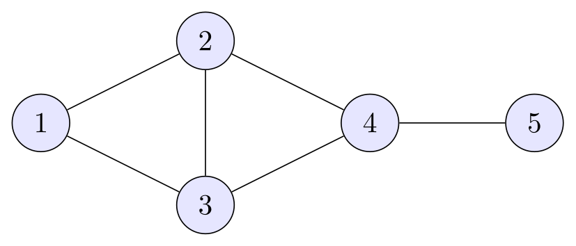
\usepackage{tikz}\begin{tikzpicture}[vertex/.style={circle, draw, fill=blue!10, minimum size=7mm}]
\node[vertex] (1) at (0,0) {1};
\node[vertex] (2) at (2,1) {2};
\node[vertex] (3) at (2,-1) {3};
\node[vertex] (4) at (4,0) {4};
\node[vertex] (5) at (6,0) {5};
\draw (1) -- (2) -- (4) -- (3) -- (1)
(2) -- (3)
(4) -- (5);
\end{tikzpicture}Full document
\documentclass[border=4pt]{standalone}
\usepackage{tikz}
\begin{document}
\begin{tikzpicture}[vertex/.style={circle, draw, fill=blue!10, minimum size=7mm}]
  \node[vertex] (1) at (0,0)    {1};
  \node[vertex] (2) at (2,1)    {2};
  \node[vertex] (3) at (2,-1)   {3};
  \node[vertex] (4) at (4,0)    {4};
  \node[vertex] (5) at (6,0)    {5};
  \draw (1) -- (2) -- (4) -- (3) -- (1)
        (2) -- (3)
        (4) -- (5);
\end{tikzpicture}
\end{document}Contents
Graphs, not plots
“Graph” means two different things in LaTeX searches. This page is about graphs in the graph-theory sense: vertices (nodes) joined by edges, as in networks, state machines, dependency graphs and trees. If you want the graph of a function or of measured data, with axes and ticks, you want pgfplots (built on TikZ, with its own manual at tikz.dev/pgfplots): \begin{axis} \addplot {x^2}; \end{axis} draws a plot with axes in two lines.
For network graphs there are three ways, from the most control to the least typing: nodes and edges placed by hand (below), the graphs library’s \graph syntax with simple automatic placement, and the graph drawing library, which computes a layout with real algorithms but needs LuaLaTeX.
Vertices and edges by hand
The picture at the top of the page is the whole technique. A style keeps the vertices consistent, vertex/.style={circle, draw, fill=blue!10, minimum size=7mm}, with minimum size so that circles with one or two digits are the same size. Each vertex gets a name in parentheses and an absolute position. A chain such as \draw (1) -- (2) -- (4) -- (3) -- (1); draws several edges at once, each from border to border, and further pieces like (2) -- (3) can follow on the same path. For dots instead of labelled circles, use circle, fill, inner sep=2pt and empty node text {}.
When the vertices follow a pattern, compute their positions. Polar coordinates (angle:radius) in a \foreach loop put vertices on a circle, and the loop can draw the edges too. The Petersen graph below has an outer pentagon at radius 2 cm and an inner star at 1 cm; \pgfmathtruncatemacro\nxt{mod(\i,5)+1} computes the index of the next vertex, wrapping from 5 back to 1, and the star joins every vertex to the one after next.
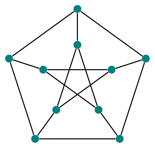
\usepackage{tikz}\begin{tikzpicture}[v/.style={circle, fill=teal, inner sep=2.2pt}]
\foreach \i in {1,...,5} {
\node[v] (o\i) at (90+72*\i-72:2cm) {}; % outer pentagon
\node[v] (i\i) at (90+72*\i-72:1cm) {}; % inner star
}
\foreach \i in {1,...,5} {
\pgfmathtruncatemacro\nxt{mod(\i,5)+1} % next vertex
\pgfmathtruncatemacro\two{mod(\i+1,5)+1} % the vertex after that
\draw[thick] (o\i) -- (o\nxt) (o\i) -- (i\i) (i\i) -- (i\two);
}
\end{tikzpicture}Full document
\documentclass[border=4pt]{standalone}
\usepackage{tikz}
\begin{document}
\begin{tikzpicture}[v/.style={circle, fill=teal, inner sep=2.2pt}]
  \foreach \i in {1,...,5} {
    \node[v] (o\i) at (90+72*\i-72:2cm) {};   % outer pentagon
    \node[v] (i\i) at (90+72*\i-72:1cm) {};   % inner star
  }
  \foreach \i in {1,...,5} {
    \pgfmathtruncatemacro\nxt{mod(\i,5)+1}    % next vertex
    \pgfmathtruncatemacro\two{mod(\i+1,5)+1}  % the vertex after that
    \draw[thick] (o\i) -- (o\nxt)  (o\i) -- (i\i)  (i\i) -- (i\two);
  }
\end{tikzpicture}
\end{document}Directed and weighted graphs
For a directed graph, add an arrow option: -> for one direction, <-> for both. With \path[->] (s) edge (a) edge (b); both edges start at s, because edge, unlike --, does not move the current point; each edge is drawn as its own path with the options of the \path. >={Stealth[round]} (arrows.meta) chooses the tip and shorten >=1pt leaves a small gap before the target.
Weights are labels on the edges. With \usetikzlibrary{quotes}, edge["4"] is short for an edge with a label node, placed with auto (the initial every edge quotes style): it goes to the left of the direction of travel, and a quote mark after it, edge["2"'], puts it on the right. The auto in the picture options does the same for labels written as node {…}. Two edges in opposite directions between the same vertices would lie on top of each other: give both bend left=20 and they curve apart, one on each side. Longhand without quotes: edge node[above] {4} or -- node[above] {4}.
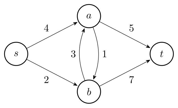
\usepackage{tikz} \usetikzlibrary{arrows.meta, quotes}\begin{tikzpicture}[>={Stealth[round]}, shorten >=1pt, auto,
v/.style={circle, draw, thick, minimum size=8mm}]
\node[v] (s) at (0,0) {$s$};
\node[v] (a) at (2.5,1.3) {$a$};
\node[v] (b) at (2.5,-1.3) {$b$};
\node[v] (t) at (5,0) {$t$};
\path[->] (s) edge["4"] (a)
edge["2"'] (b)
(a) edge["5"] (t)
edge[bend left=20, "1"] (b)
(b) edge[bend left=20, "3"] (a)
edge["7"'] (t);
\end{tikzpicture}Full document
\documentclass[border=4pt]{standalone}
\usepackage{tikz}
\usetikzlibrary{arrows.meta, quotes}
\begin{document}
\begin{tikzpicture}[>={Stealth[round]}, shorten >=1pt, auto,
    v/.style={circle, draw, thick, minimum size=8mm}]
  \node[v] (s) at (0,0)    {$s$};
  \node[v] (a) at (2.5,1.3)  {$a$};
  \node[v] (b) at (2.5,-1.3) {$b$};
  \node[v] (t) at (5,0)    {$t$};
  \path[->] (s) edge["4"]               (a)
                edge["2"']              (b)
            (a) edge["5"]               (t)
                edge[bend left=20, "1"] (b)
            (b) edge[bend left=20, "3"] (a)
                edge["7"']              (t);
\end{tikzpicture}
\end{document}Loops, parallel edges and bent edges
to[bend left=30] instead of -- curves an edge by 30° to the left of its direction (bend right the other way); with several values you get as many parallel edges as you need, as in a multigraph. out and in set the exact angles at which an edge leaves and arrives, and looseness how far it swings out.
A loop starts and ends at the same vertex. loop above, loop below, loop left and loop right set a loop with the opening on that side and place its label there, and the style every loop, initially ->, shorten >=1pt, gives it an arrow tip. Draw loops with edge, as here: an arrow tip belongs to a whole path, so a loop written \draw (a) to[loop above] (a); gets no tip, while edge makes a path of its own with the loop’s tip. The loop ignores its target, but with a named node write the node again, (a) edge[loop above] (a); the empty () of the manual’s examples only works right after a node on the same path. For other directions give the angles and then loop, in that order: edge[out=-160, in=-130, loop]. An opening of about 30° gives round loops.
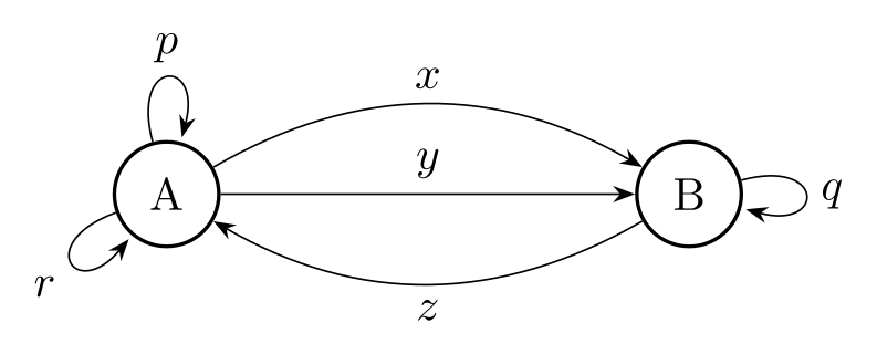
\usepackage{tikz} \usetikzlibrary{arrows.meta}\begin{tikzpicture}[>=Stealth, v/.style={circle, draw, thick, minimum size=8mm}]
\node[v] (a) at (0,0) {A};
\node[v] (b) at (4,0) {B};
% parallel edges: bent both ways and straight
\draw[->] (a) to[bend left=30] node[above] {$x$} (b);
\draw[->] (a) to node[above] {$y$} (b);
\draw[->] (b) to[bend left=30] node[below] {$z$} (a);
% loops: edge draws its own path, so every loop (->) gives it a tip
\path (a) edge[loop above] node {$p$} (a)
(b) edge[loop right] node {$q$} (b)
(a) edge[out=-160, in=-130, loop] node[below left] {$r$} (a);
\end{tikzpicture}Full document
\documentclass[border=4pt]{standalone}
\usepackage{tikz}
\usetikzlibrary{arrows.meta}
\begin{document}
\begin{tikzpicture}[>=Stealth, v/.style={circle, draw, thick, minimum size=8mm}]
  \node[v] (a) at (0,0) {A};
  \node[v] (b) at (4,0) {B};
  % parallel edges: bent both ways and straight
  \draw[->] (a) to[bend left=30] node[above] {$x$} (b);
  \draw[->] (a) to               node[above] {$y$} (b);
  \draw[->] (b) to[bend left=30] node[below] {$z$} (a);
  % loops: edge draws its own path, so every loop (->) gives it a tip
  \path (a) edge[loop above]            node {$p$} (a)
        (b) edge[loop right]            node {$q$} (b)
        (a) edge[out=-160, in=-130, loop] node[below left] {$r$} (a);
\end{tikzpicture}
\end{document}Vertex styles and highlighting a path
Styles make variations cheap. Here a source style extends the vertex style with a fill (source/.style={v, fill=green!25}), and an on path style marks the edges of a shortest path in thick red. The distances from Dijkstra’s algorithm are labels, small nodes placed outside a vertex on the side you name (label=above:3), styled once with every label. Setting every edge quotes to fill=white replaces its initial auto, so the weights sit on their edges with a white background instead of beside them.
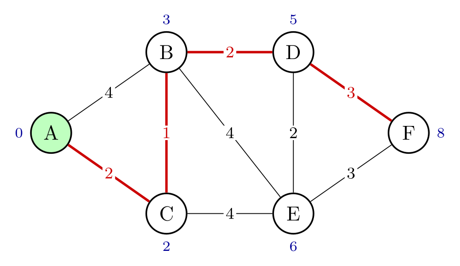
\usepackage{tikz} \usetikzlibrary{quotes}\begin{tikzpicture}[
v/.style={circle, draw, thick, fill=white, minimum size=7mm},
source/.style={v, fill=green!25},
on path/.style={very thick, red!80!black},
every edge quotes/.style={fill=white, inner sep=1pt, font=\footnotesize},
every label/.style={font=\scriptsize, text=blue!60!black}]
\node[source, label=left:0] (A) at (0,0) {A};
\node[v, label=above:3] (B) at (2,1.4) {B};
\node[v, label=below:2] (C) at (2,-1.4) {C};
\node[v, label=above:5] (D) at (4.2,1.4) {D};
\node[v, label=below:6] (E) at (4.2,-1.4){E};
\node[v, label=right:8] (F) at (6.2,0) {F};
\draw (A) edge[on path, "2"] (C) (C) edge[on path, "1"] (B)
(B) edge[on path, "2"] (D) (D) edge[on path, "3"] (F)
(A) edge["4"] (B) (C) edge["4"] (E) (B) edge["4"] (E)
(E) edge["3"] (F) (D) edge["2"] (E);
\end{tikzpicture}Full document
\documentclass[border=4pt]{standalone}
\usepackage{tikz}
\usetikzlibrary{quotes}
\begin{document}
\begin{tikzpicture}[
    v/.style={circle, draw, thick, fill=white, minimum size=7mm},
    source/.style={v, fill=green!25},
    on path/.style={very thick, red!80!black},
    every edge quotes/.style={fill=white, inner sep=1pt, font=\footnotesize},
    every label/.style={font=\scriptsize, text=blue!60!black}]
  \node[source, label=left:0]  (A) at (0,0)     {A};
  \node[v, label=above:3]      (B) at (2,1.4)   {B};
  \node[v, label=below:2]      (C) at (2,-1.4)  {C};
  \node[v, label=above:5]      (D) at (4.2,1.4) {D};
  \node[v, label=below:6]      (E) at (4.2,-1.4){E};
  \node[v, label=right:8]      (F) at (6.2,0)   {F};
  \draw (A) edge[on path, "2"] (C)  (C) edge[on path, "1"] (B)
        (B) edge[on path, "2"] (D)  (D) edge[on path, "3"] (F)
        (A) edge["4"] (B)  (C) edge["4"] (E)  (B) edge["4"] (E)
        (E) edge["3"] (F)  (D) edge["2"] (E);
\end{tikzpicture}
\end{document}The graphs library: \graph { a -> b -> c; }
\usetikzlibrary{graphs} adds a compact syntax inspired by the DOT format of Graphviz. \graph { a -> b -> c; } creates three nodes whose text is their name and joins them; a name seen again refers to the same node. The edge kinds are ->, -- (undirected), <-, <-> and -!- (no edge). Curly braces make a group: start -> {parse, validate} -> merge joins start to both and both to merge. Options after an edge kind style that edge, ->[bend left=50, "skip", dashed], where any key the graphs library does not know is passed to the edge, and the quoted label needs the quotes library.
The library also places the nodes, but only simply: grow right sep=10mm puts the nodes of a chain in a row with 10 mm between them, branch down sep=5mm stacks the members of a group, and clockwise puts the nodes on a circle. Names with spaces work (raw data); names with commas, maths or other special characters need quotes, "$x_1$" -> "$x_2$", and x1/$x_1$ gives a node the name x1 and the text x1.
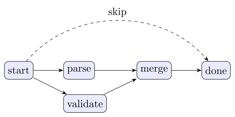
\usepackage{tikz} \usetikzlibrary{graphs, quotes, arrows.meta}\begin{tikzpicture}[>=Stealth]
\graph [grow right sep=10mm, branch down sep=5mm,
nodes={draw, rounded corners, fill=blue!8, minimum height=6mm}] {
start -> {parse, validate} -> merge -> done;
start ->[bend left=50, "skip", dashed] done;
};
\end{tikzpicture}Full document
\documentclass[border=4pt]{standalone}
\usepackage{tikz}
\usetikzlibrary{graphs, quotes, arrows.meta}
\begin{document}
\begin{tikzpicture}[>=Stealth]
  \graph [grow right sep=10mm, branch down sep=5mm,
          nodes={draw, rounded corners, fill=blue!8, minimum height=6mm}] {
    start -> {parse, validate} -> merge -> done;
    start ->[bend left=50, "skip", dashed] done;
  };
\end{tikzpicture}
\end{document}Standard graphs: K_n, C_n, K_{n,m}
\usetikzlibrary{graphs.standard} defines the common named graphs as graph macros: subgraph K_n (complete graph), subgraph C_n (cycle), subgraph P_n (path), subgraph I_n (independent set), subgraph K_nm and subgraph I_nm (complete bipartite and two independent sets) and subgraph Grid_n. n=5 is short for the vertex list V={1,...,5}; m or W={…} gives the second side of a bipartite graph. clockwise with radius=1.1cm puts the vertices on a circle (without a number, it uses the number of vertices of the subgraph), empty nodes drops the vertex labels, and each graph is moved with a scope.
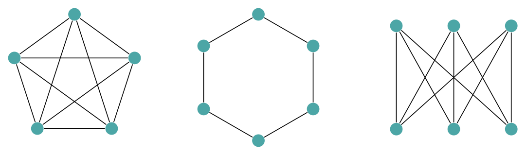
\usepackage{tikz} \usetikzlibrary{graphs.standard}\begin{tikzpicture}[every node/.style={circle, fill=teal!70, inner sep=2.2pt}]
\graph [clockwise, radius=1.1cm, empty nodes] { subgraph K_n [n=5] };
\begin{scope}[xshift=3.2cm]
\graph [clockwise, radius=1.1cm, empty nodes] { subgraph C_n [n=6] };
\end{scope}
\begin{scope}[xshift=5.6cm, yshift=0.9cm]
\graph [branch right=1cm, grow down=1.8cm, empty nodes]
{ subgraph K_nm [n=3, m=3] };
\end{scope}
\end{tikzpicture}Full document
\documentclass[border=4pt]{standalone}
\usepackage{tikz}
\usetikzlibrary{graphs.standard}
\begin{document}
\begin{tikzpicture}[every node/.style={circle, fill=teal!70, inner sep=2.2pt}]
  \graph [clockwise, radius=1.1cm, empty nodes] { subgraph K_n [n=5] };
  \begin{scope}[xshift=3.2cm]
    \graph [clockwise, radius=1.1cm, empty nodes] { subgraph C_n [n=6] };
  \end{scope}
  \begin{scope}[xshift=5.6cm, yshift=0.9cm]
    \graph [branch right=1cm, grow down=1.8cm, empty nodes]
      { subgraph K_nm [n=3, m=3] };
  \end{scope}
\end{tikzpicture}
\end{document}Automatic layouts with the graph drawing library (LuaLaTeX)
Placing vertices by hand gets slow beyond a dozen vertices. The graph drawing system computes positions with real layout algorithms, written in Lua, so it only works with LuaLaTeX; under pdfLaTeX it stops with “You need to run LuaTeX to use the graph drawing library.” Load \usetikzlibrary{graphdrawing}, then the algorithms you need with \usegdlibrary{…}, and add a layout key to the graph:
| Layout key | \usegdlibrary | Good for |
|---|---|---|
layered layout | layered | Directed acyclic graphs, flows, dependencies (Sugiyama method) |
spring layout, spring electrical layout | force | Undirected networks; clusters and symmetry show up by themselves |
tree layout, binary tree layout | trees | Trees without overlaps (Reingold–Tilford) |
simple necklace layout | circular | Nodes on a circle in the given order |
The layered layout puts each node in a layer below its predecessors and routes long edges around the others; level distance and sibling distance set the spacing. The layouts also work with nodes and edges written by hand (\node and edge inside a \tikz[spring layout] scope), not only with \graph. Force layouts start from random positions with a fixed seed (random seed, initially 42), so the same code gives the same picture on one installation; another seed gives another arrangement. The manual warns that the result can still change between LuaTeX versions, because Lua’s random number generator has changed, so when the exact placement matters, prefer a layered or tree layout or place the nodes yourself.
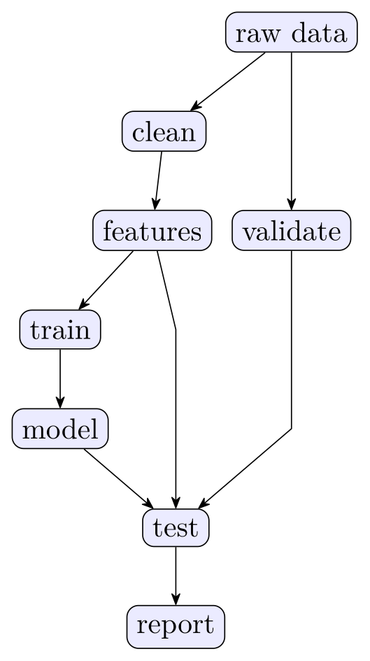
\usepackage{tikz} \usetikzlibrary{graphs, graphdrawing, arrows.meta} \usegdlibrary{layered}Compile with LuaLaTeX\begin{tikzpicture}[>={Stealth[round]}]
\graph [layered layout, level distance=12mm, sibling distance=14mm,
nodes={draw, rounded corners, fill=blue!8}] {
raw data -> {clean, validate};
clean -> features -> {train, test};
validate -> test;
train -> model -> test -> report;
};
\end{tikzpicture}Full document
\documentclass[border=4pt]{standalone}
\usepackage{tikz}
\usetikzlibrary{graphs, graphdrawing, arrows.meta}
\usegdlibrary{layered}
\begin{document}
\begin{tikzpicture}[>={Stealth[round]}]
  \graph [layered layout, level distance=12mm, sibling distance=14mm,
          nodes={draw, rounded corners, fill=blue!8}] {
    raw data -> {clean, validate};
    clean -> features -> {train, test};
    validate -> test;
    train -> model -> test -> report;
  };
\end{tikzpicture}
\end{document}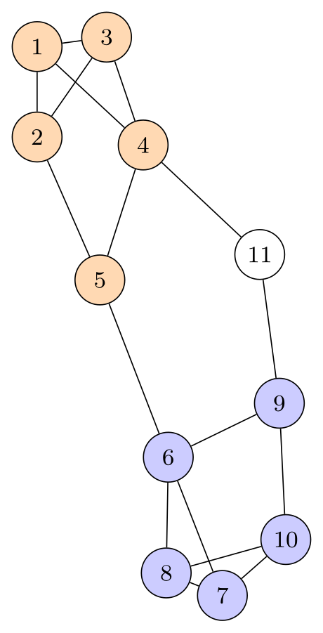
\usepackage{tikz} \usetikzlibrary{graphs, graphdrawing} \usegdlibrary{force}Compile with LuaLaTeX\begin{tikzpicture}
\graph [spring electrical layout, node distance=12mm,
nodes={circle, draw, minimum size=6mm, inner sep=0pt, font=\footnotesize}] {
{ [nodes={fill=orange!30}] 1 -- {2, 3, 4}, 2 -- {3, 5}, 3 -- 4, 4 -- 5 };
{ [nodes={fill=blue!20}] 6 -- {7, 8, 9}, 7 -- {8, 10}, 8 -- 10, 9 -- 10 };
5 -- 6;
4 -- 11 -- 9;
};
\end{tikzpicture}Full document
\documentclass[border=4pt]{standalone}
\usepackage{tikz}
\usetikzlibrary{graphs, graphdrawing}
\usegdlibrary{force}
\begin{document}
\begin{tikzpicture}
  \graph [spring electrical layout, node distance=12mm,
          nodes={circle, draw, minimum size=6mm, inner sep=0pt, font=\footnotesize}] {
    { [nodes={fill=orange!30}] 1 -- {2, 3, 4}, 2 -- {3, 5}, 3 -- 4, 4 -- 5 };
    { [nodes={fill=blue!20}]   6 -- {7, 8, 9}, 7 -- {8, 10}, 8 -- 10, 9 -- 10 };
    5 -- 6;
    4 -- 11 -- 9;
  };
\end{tikzpicture}
\end{document}State diagrams (automata)
Finite automata and state machines are graphs with conventions, and the automata library supplies them: state for a circular state, initial for the start arrow (labelled “start”; change it with initial text=… or remove it with initial text=) and accepting for the double circle. With positioning and on grid, right=of q0 measures 2.4 cm (the node distance) from centre to centre, so the states line up regardless of their size. The transitions are edges with labels placed by auto, loops for self-transitions, and bend left for the ways back.
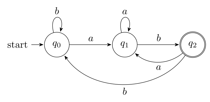
\usepackage{tikz} \usetikzlibrary{automata, positioning, arrows.meta}\begin{tikzpicture}[>={Stealth[round]}, shorten >=1pt, auto,
node distance=2.4cm, on grid]
\node[state, initial] (q0) {$q_0$};
\node[state] (q1) [right=of q0] {$q_1$};
\node[state, accepting] (q2) [right=of q1] {$q_2$};
\path[->] (q0) edge node {$a$} (q1)
edge [loop above] node {$b$} ()
(q1) edge node {$b$} (q2)
edge [loop above] node {$a$} ()
(q2) edge [bend left=40] node {$a$} (q1)
edge [bend left=55] node {$b$} (q0);
\end{tikzpicture}Full document
\documentclass[border=4pt]{standalone}
\usepackage{tikz}
\usetikzlibrary{automata, positioning, arrows.meta}
\begin{document}
\begin{tikzpicture}[>={Stealth[round]}, shorten >=1pt, auto,
                    node distance=2.4cm, on grid]
  \node[state, initial]   (q0)               {$q_0$};
  \node[state]            (q1) [right=of q0] {$q_1$};
  \node[state, accepting] (q2) [right=of q1] {$q_2$};
  \path[->] (q0) edge                node {$a$} (q1)
                 edge [loop above]   node {$b$} ()
            (q1) edge                node {$b$} (q2)
                 edge [loop above]   node {$a$} ()
            (q2) edge [bend left=40] node {$a$} (q1)
                 edge [bend left=55] node {$b$} (q0);
\end{tikzpicture}
\end{document}Common errors and how to fix them
| LaTeX says (or you see) | Cause and fix |
|---|---|
| Package tikz Error: You need to say \usetikzlibrary{graphs} in order to use the graph syntax. | The \graph command needs \usetikzlibrary{graphs}; the named graphs (subgraph K_n…) need graphs.standard. |
| Package pgf Error: You need to run LuaTeX to use the graph drawing library. | graphdrawing only works under LuaLaTeX. Compile with lualatex (on Overleaf: Menu, Compiler, LuaLaTeX), or place the nodes yourself. |
| Package pgfkeys Error: I do not know the key '/tikz/graphs/layered layout' and I am going to ignore it. Perhaps you misspelled it. | The layout key exists only after its algorithm library is loaded: \usegdlibrary{layered} for layered layout, force for spring layouts, trees for tree layout, circular for simple necklace layout. |
| Package pgfkeys Error: I do not know the key '/tikz/"4"' and I am going to ignore it. Perhaps you misspelled it. | Quoted labels such as edge["4"] need \usetikzlibrary{quotes}. Without it, write edge node[above] {4}. |
| Extra }, or forgotten $. | A \graph node name contains maths or a comma, as in $x_1$ -> $x_2, x_3$. Put such names in quotes: "$x_1$" -> "$x_2, x_3$", or use name/text: x1/$x_1$. |
| Package pgf Error: No shape named `' is known. | A loop written (a) edge[loop above] node {p} (); the empty () only works directly after a node on the same path. Repeat the node name as the target: (a) edge[loop above] node {p} (a). |
| A loop has no arrow tip, or comes out as a tiny curl (no error) | Arrow tips belong to whole paths: draw loops with edge (each edge is its own path and gets every loop’s ->), not with \draw … to[loop above]. With custom angles, put loop last: edge[out=-160, in=-130, loop]; in and out given after loop turn it back into an ordinary curve. |
Frequently asked questions
How do I draw a graph with vertices and edges in TikZ?
Define a vertex style (circle, draw, minimum size=7mm), place named nodes with \node[vertex] (a) at (0,0) {a};, and draw the edges with \draw (a) -- (b); or \path (a) edge (b) edge (c);. The lines stop at the node borders automatically. For many vertices on a circle, use polar coordinates in a \foreach loop.
How do I draw a directed weighted graph in TikZ?
Use -> on the edges and put the weight in a label: with \usetikzlibrary{quotes}, \path[->] (a) edge["5"] (b);, together with auto so that labels sit beside the edges. For edges in both directions between two vertices, give both bend left=20 so that they curve apart.
How do I draw a self-loop in TikZ?
Use an edge with a loop style on the node itself: \path (a) edge[loop above] node {x} (a);. loop below, loop left and loop right work the same way, and for another direction write edge[out=-150, in=-120, loop] with loop last. every loop gives it an arrow tip.
Does TikZ have automatic graph layout?
Yes, the graph drawing library: \usetikzlibrary{graphdrawing} plus \usegdlibrary{layered, force, trees, circular}, and a key such as layered layout or spring electrical layout on the graph. It runs Lua code, so it needs LuaLaTeX; pdfLaTeX stops with "You need to run LuaTeX to use the graph drawing library." Without LuaLaTeX, the graphs library offers only simple placement (grow right, branch down, clockwise).
How do I draw a complete graph K_n in TikZ?
Load \usetikzlibrary{graphs.standard} and write \graph[clockwise, radius=1.2cm] { subgraph K_n [n=6] };. C_n, P_n, K_nm and Grid_n work the same way. By hand, place n nodes on a circle with \foreach and join every pair with two nested loops.
How do I draw a function graph in LaTeX?
That is a plot, not a graph of vertices and edges: use pgfplots, for example \begin{tikzpicture}\begin{axis} \addplot[domain=-2:2] {x^2}; \end{axis}\end{tikzpicture} with \usepackage{pgfplots}. Plain TikZ can also plot with \draw plot, but pgfplots handles axes, ticks and legends for you.
References
- PGF/TikZ manual, §17.12 Connecting Nodes: Using the Edge Operationtikz.dev
- PGF/TikZ manual, §17.10.4 The Quotes Syntaxtikz.dev
- PGF/TikZ manual, §74.3 To Path Library: Curves (bend, in, out, looseness)tikz.dev
- PGF/TikZ manual, §74.4 To Path Library: Loopstikz.dev
- PGF/TikZ manual, §19 Specifying Graphs (the graphs library)tikz.dev
- PGF/TikZ manual, §19.3.3 Syntax of Chain Specifications (edge kinds)tikz.dev
- PGF/TikZ manual, §19.9 Online Placement Strategiestikz.dev
- PGF/TikZ manual, §19.10.1 Graph Macros (graphs.standard)tikz.dev
- PGF/TikZ manual, §27 Introduction to Algorithmic Graph Drawingtikz.dev
- PGF/TikZ manual, §28.1 Choosing a Layout and a Librarytikz.dev
- PGF/TikZ manual, §31 Graph Drawing Algorithms: Layered Layoutstikz.dev
- PGF/TikZ manual, §32 Graph Drawing Algorithms: Force-Based Methodstikz.dev
- PGF/TikZ manual, §43 Automata Drawing Librarytikz.dev
- pgf package (TikZ) 3.1.12 on CTAN, with the full manual as PDFctan.org
The facts on this page were checked against these sources, and every picture is the code with it typeset with TeX Live 2026. Code on this page: CC0 1.0, copy it freely.
Try the code in your browserEvery snippet on this page opens in the free TikZ editor: it is typeset with TeX Live as you type, with errors pointed at their line.
Open the TikZ editor