TikZ diagrams: block, cycle, flowchart, tree and more
Quick answer
\node[draw] (a) {Text};), placed next to each other with the positioning library (right=of a), joined by arrows (\draw[->] (a) -- (b);, which stop at the node borders), and grouped with fit and backgrounds. Block diagrams and flowcharts are exactly that; cycle diagrams add polar coordinates and \foreach; trees, graphs, matrices, commutative diagrams and circuits have dedicated syntax or packages, each shown below with a link to its full guide.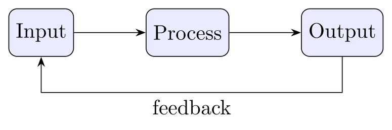
\usepackage{tikz} \usetikzlibrary{positioning, arrows.meta}\begin{tikzpicture}[node distance=12mm, >=Stealth,
box/.style={draw, rounded corners, fill=blue!8, minimum height=8mm}]
\node[box] (in) {Input};
\node[box, right=of in] (proc) {Process};
\node[box, right=of proc] (out) {Output};
\draw[->] (in) -- (proc);
\draw[->] (proc) -- (out);
\draw[->] (out.south) -- ++(0,-6mm) -| node[pos=0.25, below] {feedback} (in.south);
\end{tikzpicture}Full document
\documentclass[border=4pt]{standalone}
\usepackage{tikz}
\usetikzlibrary{positioning, arrows.meta}
\begin{document}
\begin{tikzpicture}[node distance=12mm, >=Stealth,
    box/.style={draw, rounded corners, fill=blue!8, minimum height=8mm}]
  \node[box]               (in)   {Input};
  \node[box, right=of in]  (proc) {Process};
  \node[box, right=of proc] (out) {Output};
  \draw[->] (in) -- (proc);
  \draw[->] (proc) -- (out);
  \draw[->] (out.south) -- ++(0,-6mm) -| node[pos=0.25, below] {feedback} (in.south);
\end{tikzpicture}
\end{document}Contents
The building blocks: nodes, positioning, arrows and groups
Almost any diagram reduces to four steps, and the snippet at the top uses all of them except the last:
- Nodes.
\node[draw, rounded corners] (in) {Input};makes a box namedin. The shape (rectangleby default,circle,ellipse, ordiamondandtrapeziumfromshapes.geometric), its size (minimum width,minimum height) and its text (align=centerfor several lines,text widthto wrap) are options. Define the look once as a style,box/.style={…}, and every node uses[box]. - Positions. Either give coordinates (
at (3,0)), or place nodes relative to each other with\usetikzlibrary{positioning}:right=of inleaves exactly thenode distancebetween the two borders (initially 1 cm),below=5mm of inoverrides it, andnode distance=8mm and 12mmsets the vertical and horizontal gaps separately. Grids of nodes are easier with a matrix, circles of nodes with polar coordinates(90:2cm)in a\foreachloop. - Connections.
\draw[->] (a) -- (b);draws from border to border;-|goes horizontally then vertically and|-the other way, which is how feedback loops and flowchart branches get their right angles. A node on the path labels it:-- node[above] {yes}. Arrow tips come fromarrows.meta, see TikZ arrows. - Groups.
fit=(a) (b)(libraryfit) makes a node just big enough to contain other nodes, and\begin{scope}[on background layer](librarybackgrounds) draws it behind them, so the frame and its fill do not cover the boxes it groups.
| Library | What it adds |
|---|---|
positioning | right=of a, below=1cm of a, node distance between borders, on grid |
arrows.meta | Arrow tips with options: Stealth, Latex, -{Stealth[length=3mm]} |
shapes.geometric, shapes.misc | diamond, trapezium, ellipse, cylinder; rounded rectangle |
fit, backgrounds | Frames around groups of nodes, drawn on a layer behind them |
calc | Computed points such as ($(a)!0.5!(b)$), halfway between two nodes |
matrix, chains, quotes | Grids of nodes, nodes in a row joined automatically, edge["label"] |
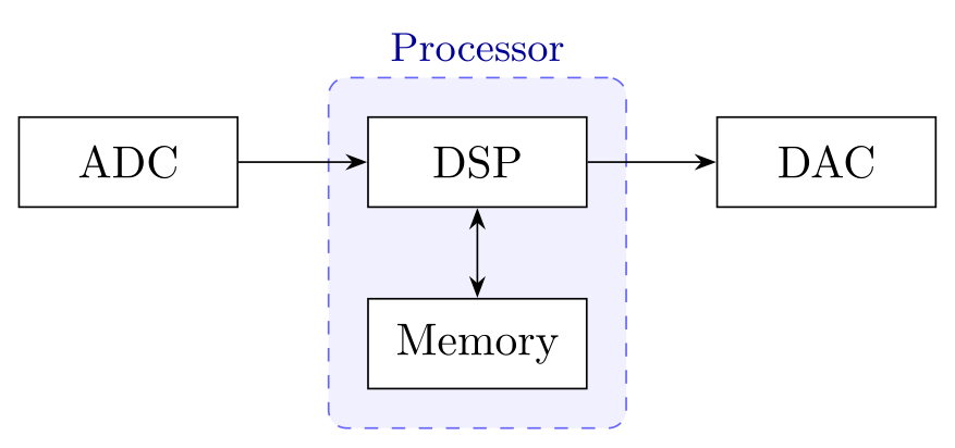
\usepackage{tikz} \usetikzlibrary{positioning, fit, backgrounds, arrows.meta}\begin{tikzpicture}[>=Stealth, node distance=7mm and 10mm,
box/.style={draw, fill=white, minimum width=17mm, minimum height=7mm}]
\node[box] (adc) {ADC};
\node[box, right=of adc] (dsp) {DSP};
\node[box, below=of dsp] (mem) {Memory};
\node[box, right=of dsp] (dac) {DAC};
\draw[->] (adc) -- (dsp);
\draw[->] (dsp) -- (dac);
\draw[<->] (dsp) -- (mem);
\begin{scope}[on background layer]
\node[draw=blue!60, dashed, fill=blue!6, rounded corners, inner sep=3mm,
fit=(dsp) (mem), label={[blue!60!black, font=\small]above:Processor}] {};
\end{scope}
\end{tikzpicture}Full document
\documentclass[border=4pt]{standalone}
\usepackage{tikz}
\usetikzlibrary{positioning, fit, backgrounds, arrows.meta}
\begin{document}
\begin{tikzpicture}[>=Stealth, node distance=7mm and 10mm,
    box/.style={draw, fill=white, minimum width=17mm, minimum height=7mm}]
  \node[box]               (adc) {ADC};
  \node[box, right=of adc] (dsp) {DSP};
  \node[box, below=of dsp] (mem) {Memory};
  \node[box, right=of dsp] (dac) {DAC};
  \draw[->]  (adc) -- (dsp);
  \draw[->]  (dsp) -- (dac);
  \draw[<->] (dsp) -- (mem);
  \begin{scope}[on background layer]
    \node[draw=blue!60, dashed, fill=blue!6, rounded corners, inner sep=3mm,
          fit=(dsp) (mem), label={[blue!60!black, font=\small]above:Processor}] {};
  \end{scope}
\end{tikzpicture}
\end{document}Block diagrams
A block diagram is nodes and arrows with three extras: open ends, summing junctions and branch points. An input or output that has no box is a \coordinate, which positioning can place like a node (\coordinate[right=6mm of plant] (branch);). The summing junction is a small empty circle node, with the signs as tiny nodes beside it, and the branch point is a filled dot drawn at the coordinate. The feedback path uses the right-angle connectors: (branch) |- (sensor) goes down and then left into the sensor, (sensor) -| (sum) goes left and then up into the junction.
node distance=8mm and 10mm gives 8 mm between rows and 10 mm between columns, so every arrow has room for its signal label (node[above] {$u$}). The sensor is placed with below=of ctrl.south east: when the part after of is a point (here an anchor) rather than a node name, the new node is placed node distance below that point, so the sensor is centred under the controller’s right edge, between the two blocks.
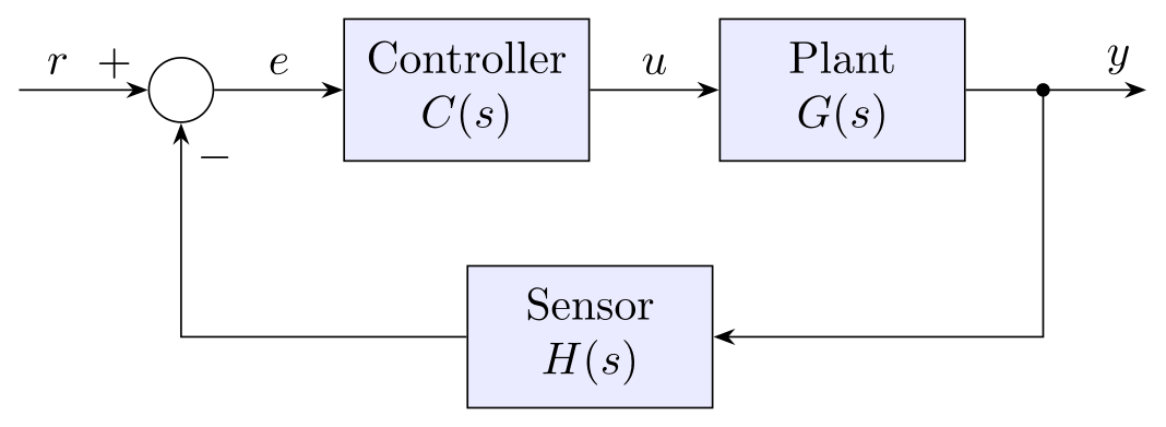
\usepackage{tikz} \usetikzlibrary{positioning, arrows.meta}\begin{tikzpicture}[>=Stealth, node distance=8mm and 10mm,
block/.style={draw, fill=blue!8, minimum width=19mm, minimum height=11mm, align=center},
sum/.style={draw, circle, minimum size=5mm, inner sep=0pt}]
\coordinate (r);
\node[sum, right=of r] (sum) {};
\node[block, right=of sum] (ctrl) {Controller\\$C(s)$};
\node[block, right=of ctrl] (plant) {Plant\\$G(s)$};
\coordinate[right=6mm of plant] (branch);
\coordinate[right=8mm of branch] (y);
\node[block, below=of ctrl.south east] (sensor) {Sensor\\$H(s)$};
\draw[->] (r) -- node[above, pos=0.3] {$r$} (sum);
\draw[->] (sum) -- node[above] {$e$} (ctrl);
\draw[->] (ctrl) -- node[above] {$u$} (plant);
\draw[->] (plant) -- (y) node[above left] {$y$};
\fill (branch) circle[radius=1.5pt];
\draw[->] (branch) |- (sensor);
\draw[->] (sensor) -| node[pos=0.92, right] {$-$} (sum);
\node[above left=-1pt and 0pt of sum.west] {$+$};
\end{tikzpicture}Full document
\documentclass[border=4pt]{standalone}
\usepackage{tikz}
\usetikzlibrary{positioning, arrows.meta}
\begin{document}
\begin{tikzpicture}[>=Stealth, node distance=8mm and 10mm,
    block/.style={draw, fill=blue!8, minimum width=19mm, minimum height=11mm, align=center},
    sum/.style={draw, circle, minimum size=5mm, inner sep=0pt}]
  \coordinate (r);
  \node[sum, right=of r]        (sum)    {};
  \node[block, right=of sum]    (ctrl)   {Controller\\$C(s)$};
  \node[block, right=of ctrl]   (plant)  {Plant\\$G(s)$};
  \coordinate[right=6mm of plant] (branch);
  \coordinate[right=8mm of branch] (y);
  \node[block, below=of ctrl.south east] (sensor) {Sensor\\$H(s)$};

  \draw[->] (r) -- node[above, pos=0.3] {$r$} (sum);
  \draw[->] (sum) -- node[above] {$e$} (ctrl);
  \draw[->] (ctrl) -- node[above] {$u$} (plant);
  \draw[->] (plant) -- (y) node[above left] {$y$};
  \fill (branch) circle[radius=1.5pt];
  \draw[->] (branch) |- (sensor);
  \draw[->] (sensor) -| node[pos=0.92, right] {$-$} (sum);
  \node[above left=-1pt and 0pt of sum.west] {$+$};
\end{tikzpicture}
\end{document}Cycle diagrams
A cycle diagram places the stages on a circle and joins them with curved arrows. Both come from polar coordinates: (\a:\r) is the point at angle \a (degrees, counter-clockwise from the right) and distance \r from the origin. The loop gives stage \i the angle 90 - 360/\n*(\i-1), so the first stage sits at the top and the others follow clockwise; \pgfmathsetmacro computes it once per stage.
Each arrow is an arc on the same circle that starts \gap degrees after one stage and ends \gap degrees before the next, so it never runs into the nodes: arc[start angle=\a-\gap, end angle=\a-360/\n+\gap, radius=\r]. An end angle smaller than the start angle draws clockwise. To change the number of stages, change \n and the list; if the nodes get closer together, increase \gap or \r. The stage style takes the colour as a parameter (stage/.style={… draw=#1!70!black, fill=#1!15}), and the fixed minimum size with a text width keeps all the circles equal, whatever their text.
For a quick result without any geometry, the smartdiagram package (version 0.3b) draws a coloured cycle from a list: \smartdiagram[circular diagram:clockwise]{Observe, Ask a question, Hypothesis, Experiment, Analyse}. It is a command rather than an environment, its boxes have a fixed width (long words are hyphenated) and changing its look means learning its own options, so the hand-made version above is the more flexible one.
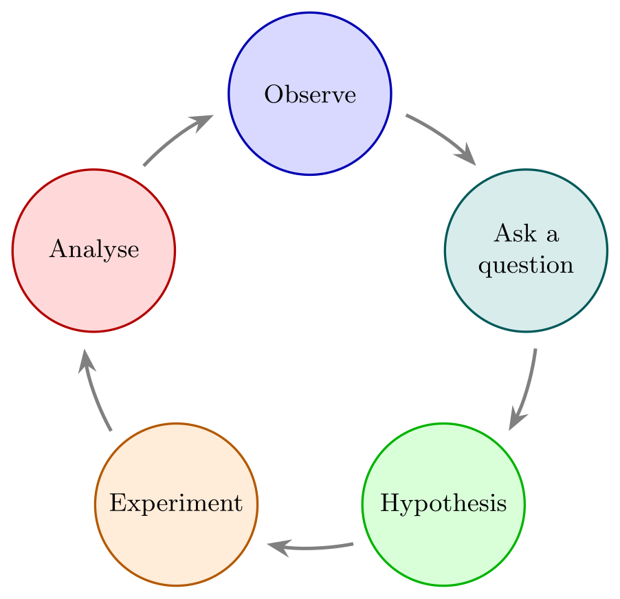
\usepackage{tikz} \usetikzlibrary{arrows.meta}\begin{tikzpicture}[>={Stealth[length=3mm]},
stage/.style={circle, draw=#1!70!black, fill=#1!15, thick, minimum size=20mm,
inner sep=0pt, text width=17mm, align=center, font=\small}]
\def\n{5} % number of stages
\def\r{2.8cm} % radius of the cycle
\def\gap{25} % degrees kept free around each stage
\foreach \text/\col [count=\i] in {Observe/blue, Ask a\\question/teal,
Hypothesis/green, Experiment/orange, Analyse/red} {
\pgfmathsetmacro\a{90 - 360/\n*(\i-1)} % clockwise from the top
\node[stage=\col] at (\a:\r) {\text};
\draw[->, very thick, gray] (\a-\gap:\r)
arc[start angle=\a-\gap, end angle=\a-360/\n+\gap, radius=\r];
}
\end{tikzpicture}Full document
\documentclass[border=4pt]{standalone}
\usepackage{tikz}
\usetikzlibrary{arrows.meta}
\begin{document}
\begin{tikzpicture}[>={Stealth[length=3mm]},
    stage/.style={circle, draw=#1!70!black, fill=#1!15, thick, minimum size=20mm,
                  inner sep=0pt, text width=17mm, align=center, font=\small}]
  \def\n{5}      % number of stages
  \def\r{2.8cm}  % radius of the cycle
  \def\gap{25}   % degrees kept free around each stage
  \foreach \text/\col [count=\i] in {Observe/blue, Ask a\\question/teal,
      Hypothesis/green, Experiment/orange, Analyse/red} {
    \pgfmathsetmacro\a{90 - 360/\n*(\i-1)}   % clockwise from the top
    \node[stage=\col] at (\a:\r) {\text};
    \draw[->, very thick, gray] (\a-\gap:\r)
      arc[start angle=\a-\gap, end angle=\a-360/\n+\gap, radius=\r];
  }
\end{tikzpicture}
\end{document}Flowcharts
A flowchart is a block diagram with standard shapes: rounded terminators for start and end, rectangles for steps, a diamond (shapes.geometric, with aspect=2 to make it wide and flat) for decisions, and a slanted trapezium for input and output. The yes and no labels are nodes on the arrows, and |- brings a side branch back into the main column. The TikZ flowchart guide has the full set of shapes, a reusable template, loops and swimlanes.
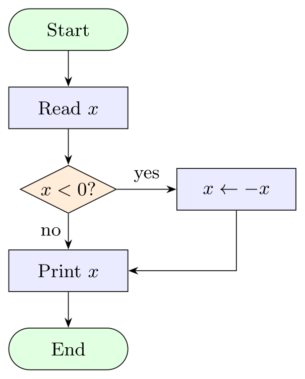
\usepackage{tikz} \usetikzlibrary{shapes.geometric, arrows.meta, positioning}\begin{tikzpicture}[node distance=6mm and 10mm, >=Stealth, font=\small,
term/.style={draw, rounded corners=3.5mm, minimum width=20mm, minimum height=7mm, fill=green!12},
proc/.style={draw, minimum width=20mm, minimum height=7mm, fill=blue!8},
dec/.style={draw, diamond, aspect=2, inner sep=1pt, fill=orange!15}]
\node[term] (start) {Start};
\node[proc, below=of start] (read) {Read $x$};
\node[dec, below=of read] (test) {$x < 0$?};
\node[proc, right=of test] (neg) {$x \gets -x$};
\node[proc, below=of test] (print) {Print $x$};
\node[term, below=of print] (stop) {End};
\draw[->] (start) -- (read);
\draw[->] (read) -- (test);
\draw[->] (test) -- node[above] {yes} (neg);
\draw[->] (test) -- node[left] {no} (print);
\draw[->] (neg) |- (print);
\draw[->] (print) -- (stop);
\end{tikzpicture}Full document
\documentclass[border=4pt]{standalone}
\usepackage{tikz}
\usetikzlibrary{shapes.geometric, arrows.meta, positioning}
\begin{document}
\begin{tikzpicture}[node distance=6mm and 10mm, >=Stealth, font=\small,
    term/.style={draw, rounded corners=3.5mm, minimum width=20mm, minimum height=7mm, fill=green!12},
    proc/.style={draw, minimum width=20mm, minimum height=7mm, fill=blue!8},
    dec/.style={draw, diamond, aspect=2, inner sep=1pt, fill=orange!15}]
  \node[term]                  (start) {Start};
  \node[proc, below=of start]  (read)  {Read $x$};
  \node[dec,  below=of read]   (test)  {$x < 0$?};
  \node[proc, right=of test]   (neg)   {$x \gets -x$};
  \node[proc, below=of test]   (print) {Print $x$};
  \node[term, below=of print]  (stop)  {End};
  \draw[->] (start) -- (read);
  \draw[->] (read) -- (test);
  \draw[->] (test) -- node[above] {yes} (neg);
  \draw[->] (test) -- node[left] {no} (print);
  \draw[->] (neg) |- (print);
  \draw[->] (print) -- (stop);
\end{tikzpicture}
\end{document}Trees, org charts and hierarchies
TikZ has a built-in child syntax for trees, but it spaces children by a fixed distance, whatever their size. For org charts and anything with labels of different widths, the forest package (version 2.1.5) is the better tool: you write the tree as nested brackets, [Director [Research …] …], and forest packs it without overlaps. for tree={…} styles every node, and forked edges from forest’s edges library draws the right-angled connectors of an org chart. The fixed text height and text depth give every box the same size, so the levels line up even when a label has a descender. Binary trees, decision trees, directory trees and tikz-qtree are on the TikZ trees page.
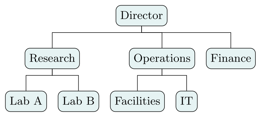
\usepackage{tikz} \usepackage{forest} \useforestlibrary{edges}\begin{forest}
for tree={draw, rounded corners, fill=teal!10, font=\small,
text height=1.7ex, text depth=0.5ex, s sep=3mm, l sep=6mm},
forked edges,
[Director
[Research [Lab A] [Lab B]]
[Operations [Facilities] [IT]]
[Finance]
]
\end{forest}Full document
\documentclass[border=4pt]{standalone}
\usepackage{tikz}
\usepackage{forest}
\useforestlibrary{edges}
\begin{document}
\begin{forest}
  for tree={draw, rounded corners, fill=teal!10, font=\small,
            text height=1.7ex, text depth=0.5ex, s sep=3mm, l sep=6mm},
  forked edges,
  [Director
    [Research [Lab A] [Lab B]]
    [Operations [Facilities] [IT]]
    [Finance]
  ]
\end{forest}
\end{document}Graphs and networks
A graph in the network sense is vertices and edges: circle nodes and lines between them. (a) edge (b) draws one edge from a path and can be repeated on the same path, and with \usetikzlibrary{quotes}, edge["4"] adds a weight. The every edge quotes style is initially auto, which puts labels beside the edge; replacing it with fill=white centres them on the edge with a white background. The TikZ graphs page covers directed and weighted graphs, loops, the \graph syntax and automatic layouts. For function plots, use pgfplots instead.
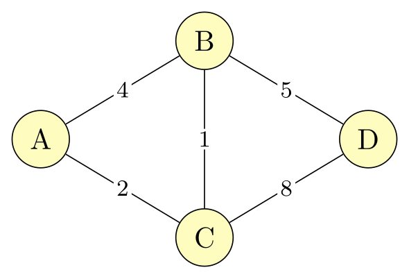
\usepackage{tikz} \usetikzlibrary{quotes}\begin{tikzpicture}[v/.style={circle, draw, fill=yellow!25, minimum size=7mm},
every edge quotes/.style={fill=white, inner sep=1pt, font=\footnotesize}]
\node[v] (a) at (0,0) {A};
\node[v] (b) at (2,1.2) {B};
\node[v] (c) at (2,-1.2) {C};
\node[v] (d) at (4,0) {D};
\draw (a) edge["4"] (b) (a) edge["2"] (c) (b) edge["1"] (c)
(b) edge["5"] (d) (c) edge["8"] (d);
\end{tikzpicture}Full document
\documentclass[border=4pt]{standalone}
\usepackage{tikz}
\usetikzlibrary{quotes}
\begin{document}
\begin{tikzpicture}[v/.style={circle, draw, fill=yellow!25, minimum size=7mm},
    every edge quotes/.style={fill=white, inner sep=1pt, font=\footnotesize}]
  \node[v] (a) at (0,0)    {A};
  \node[v] (b) at (2,1.2)  {B};
  \node[v] (c) at (2,-1.2) {C};
  \node[v] (d) at (4,0)    {D};
  \draw (a) edge["4"] (b)  (a) edge["2"] (c)  (b) edge["1"] (c)
        (b) edge["5"] (d)  (c) edge["8"] (d);
\end{tikzpicture}
\end{document}Timelines
A timeline is a line with ticks, and the ticks are a \foreach loop over position/year/event triples. x=1.8cm makes one step along the axis 1.8 cm, so the events can be numbered 0, 1, 2 and still be spread out, and text width with align=center wraps a long event name onto two lines instead of letting it collide with its neighbours. Vertical timelines, events above and below, periods and Gantt charts are on the TikZ timeline page.

\usepackage{tikz} \usetikzlibrary{arrows.meta}\begin{tikzpicture}[x=1.8cm]
\draw[thick, -Stealth] (0,0) -- (5.55,0);
\foreach \x/\year/\event in {0/2021/Idea, 1/2022/Prototype, 2/2023/First paper,
3/2024/Patent, 4/2025/Spin-off, 5/2026/Product} {
\fill[blue!70!black] (\x,0) circle[radius=2pt];
\node[below=3pt, font=\small] at (\x,0) {\year};
\node[above=3pt, font=\small, text width=1.6cm, align=center] at (\x,0) {\event};
}
\end{tikzpicture}Full document
\documentclass[border=4pt]{standalone}
\usepackage{tikz}
\usetikzlibrary{arrows.meta}
\begin{document}
\begin{tikzpicture}[x=1.8cm]
  \draw[thick, -Stealth] (0,0) -- (5.55,0);
  \foreach \x/\year/\event in {0/2021/Idea, 1/2022/Prototype, 2/2023/First paper,
                               3/2024/Patent, 4/2025/Spin-off, 5/2026/Product} {
    \fill[blue!70!black] (\x,0) circle[radius=2pt];
    \node[below=3pt, font=\small] at (\x,0) {\year};
    \node[above=3pt, font=\small, text width=1.6cm, align=center] at (\x,0) {\event};
  }
\end{tikzpicture}
\end{document}Matrices and grids
The matrix library turns a table into nodes: in a matrix of math nodes, every cell is a node in maths mode, cells are separated by & and every row ends with \\, including the last. Cells are named after the matrix, (m-2-3) for row 2, column 3, so you can draw on top of the matrix afterwards, as with the red frame around the second row. left delimiter and right delimiter add brackets of the right height, and styles such as row 2 column 2/.style colour single cells. More, including array and memory diagrams, on the TikZ matrix page.
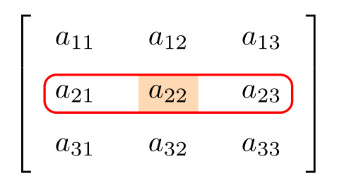
\usepackage{tikz} \usetikzlibrary{matrix}\begin{tikzpicture}
\matrix (m) [matrix of math nodes, left delimiter={[}, right delimiter={]},
row sep=2mm, column sep=4mm,
row 2 column 2/.style={nodes={fill=orange!30}}]
{
a_{11} & a_{12} & a_{13} \\
a_{21} & a_{22} & a_{23} \\
a_{31} & a_{32} & a_{33} \\
};
\draw[red, thick, rounded corners] (m-2-1.north west) rectangle (m-2-3.south east);
\end{tikzpicture}Full document
\documentclass[border=4pt]{standalone}
\usepackage{tikz}
\usetikzlibrary{matrix}
\begin{document}
\begin{tikzpicture}
  \matrix (m) [matrix of math nodes, left delimiter={[}, right delimiter={]},
               row sep=2mm, column sep=4mm,
               row 2 column 2/.style={nodes={fill=orange!30}}]
  {
    a_{11} & a_{12} & a_{13} \\
    a_{21} & a_{22} & a_{23} \\
    a_{31} & a_{32} & a_{33} \\
  };
  \draw[red, thick, rounded corners] (m-2-1.north west) rectangle (m-2-3.south east);
\end{tikzpicture}
\end{document}Commutative diagrams
Commutative diagrams have their own package, tikz-cd, which works like an array: objects separated by & and \\, and arrows given by direction letters (\arrow[r, "f"] points one cell right and is labelled f; a quote mark after the label, "g"', moves it to the other side). It is much shorter than placing the nodes by hand. See commutative diagrams in TikZ.
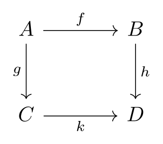
\usepackage{tikz} \usepackage{tikz-cd}\begin{tikzcd}[sep=large]
A \arrow[r, "f"] \arrow[d, "g"'] & B \arrow[d, "h"] \\
C \arrow[r, "k"'] & D
\end{tikzcd}Full document
\documentclass[border=4pt]{standalone}
\usepackage{tikz}
\usepackage{tikz-cd}
\begin{document}
\begin{tikzcd}[sep=large]
  A \arrow[r, "f"] \arrow[d, "g"'] & B \arrow[d, "h"] \\
  C \arrow[r, "k"']                & D
\end{tikzcd}
\end{document}Circuit diagrams
Electrical circuits are drawn with circuitikz, which adds components as path operations: to[R, l=$R$] draws a resistor with a label between two points, to[C] a capacitor, to[sV] a sinusoidal source, and to[short, -o] a wire ending in an open terminal. The american package option gives the zigzag resistor and the plus and minus signs of the output voltage. See CircuiTikZ for components, labels and styles.
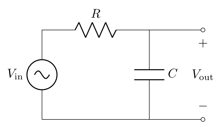
\usepackage{tikz} \usepackage[american]{circuitikz}\begin{circuitikz}
\draw (0,0) to[sV, l=$V_\mathrm{in}$] (0,2.5)
to[R, l=$R$] (3,2.5)
to[C, l=$C$] (3,0) -- (0,0);
\draw (3,2.5) to[short, -o] (4.5,2.5)
(3,0) to[short, -o] (4.5,0);
\draw (4.5,2.5) to[open, v^=$V_\mathrm{out}$] (4.5,0);
\end{circuitikz}Full document
\documentclass[border=4pt]{standalone}
\usepackage{tikz}
\usepackage[american]{circuitikz}
\begin{document}
\begin{circuitikz}
  \draw (0,0) to[sV, l=$V_\mathrm{in}$] (0,2.5)
              to[R, l=$R$] (3,2.5)
              to[C, l=$C$] (3,0) -- (0,0);
  \draw (3,2.5) to[short, -o] (4.5,2.5)
        (3,0)   to[short, -o] (4.5,0);
  \draw (4.5,2.5) to[open, v^=$V_\mathrm{out}$] (4.5,0);
\end{circuitikz}
\end{document}TikZ or a diagram maker?
TikZ is the right tool when the diagram belongs in a LaTeX document: it uses the document’s fonts and maths, it is exact (every distance is a number you chose), it stays in your source with the text and under version control, and changing one style restyles every diagram. The cost is that you see the result only after compiling, and arranging a large diagram by coordinates takes time. Some ways to work faster:
- A live TikZ editor. The LabCanvas TikZ editor typesets your code with TeX Live as you pause typing and points errors to their line, so you can adjust numbers and see the result at once. It downloads PNG images (300 or 600 dpi), not code generated from drawing: you still write the TikZ. Note that it preloads common libraries, so add the
\usetikzlibrarylines when you copy code into your own document (every snippet on this page lists them). - Graphical editors that save TikZ. TikZiT draws node-and-edge graphs and string diagrams with the mouse and saves them as TikZ; quiver does the same for commutative diagrams and exports tikz-cd.
- A visual figure editor. For illustrations rather than diagrams of boxes and arrows (cells, lab setups, graphical abstracts), a drag-and-drop editor is quicker than code. The LabCanvas figure editor is one: a TikZ figure from the TikZ editor can be opened in it as editable shapes and combined with other panels. It does not write TikZ code, and its exports are part of LabCanvas Pro (it is free to use with up to 3 designs).
Common errors and how to fix them
| LaTeX says (or you see) | Cause and fix |
|---|---|
| Package PGF Math Error: Unknown function `of' (in 'of a'). | right=of a was used without the positioning library, so TikZ reads "of a" as a length. Add \usetikzlibrary{positioning}. |
| Package pgfkeys Error: I do not know the key '/tikz/fit', to which you passed '(a) (b)', and I am going to ignore it. Perhaps you misspelled it. | fit is in a library: add \usetikzlibrary{fit}. |
| Package pgfkeys Error: I do not know the key '/tikz/on background layer' and I am going to ignore it. Perhaps you misspelled it. | The background layer comes from \usetikzlibrary{backgrounds}. |
| Package pgf Error: No shape named `c' is known. | An arrow refers to a node name that does not exist (yet): check the spelling, and draw arrows only after both nodes are defined. Names are case-sensitive. |
| Line breaks in a node are ignored: Controller\\$C(s)$ prints “ControllerC(s)” (no error) | A node only breaks lines when it knows how to align them: add align=center (or left, right), or a text width. |
| Arrows or frames are drawn on top of the boxes (no error) | Whatever is drawn later covers what was drawn earlier. Draw the frames first or put them in \begin{scope}[on background layer]; give boxes a fill so that lines behind them are hidden. |
Frequently asked questions
How do I draw a block diagram in TikZ?
Load \usetikzlibrary{positioning, arrows.meta}, define a block style (draw, minimum width, minimum height), place the blocks with right=of and below=of, and connect them with \draw[->] (a) -- (b);. Use a small circle node for a summing junction, a \coordinate for open inputs and outputs, and |- or -| for feedback paths with right angles.
How do I make a cycle diagram in LaTeX?
Place the stages at polar coordinates in a \foreach loop, for example at (90-360/5*(\i-1):2.8cm) for five stages clockwise from the top, and draw each arrow as an arc on the same circle that starts and ends a few degrees away from the stages. For a ready-made look with less control, \smartdiagram[circular diagram:clockwise]{A, B, C} from the smartdiagram package draws a cycle from a list.
Is there a TikZ diagram maker with a graphical interface?
TikZiT (graphs and string diagrams) and quiver (commutative diagrams) let you draw with the mouse and save TikZ code. For other diagrams you write the code, but a live editor such as the LabCanvas TikZ editor shows the result as you type, which makes adjusting positions quick.
How do I put a box around a group of nodes?
Load the fit library and add a node with fit=(a) (b) (c) and draw, dashed or rounded corners as you like; inner sep sets the margin. Put it inside \begin{scope}[on background layer] (backgrounds library) so its fill stays behind the grouped nodes, and give it a label with label=above:Name.
Which TikZ libraries do I need for diagrams?
Usually positioning (relative placement), arrows.meta (arrow tips) and shapes.geometric (diamond, trapezium, ellipse). Add fit and backgrounds for frames around groups, calc for computed points, matrix for grids of nodes and quotes for short edge labels. Trees, commutative diagrams and circuits use the forest, tikz-cd and circuitikz packages.
How do I get a TikZ diagram into Word or PowerPoint?
Compile it on its own with \documentclass[border=4pt]{standalone} to get a PDF of just the diagram, then convert that to PNG, or paste the code into an online TikZ editor and download a PNG at 300 or 600 dpi.
References
- PGF/TikZ manual, §5 Tutorial: Diagrams as Simple Graphstikz.dev
- PGF/TikZ manual, §17.5.3 Advanced Placement Options (positioning library)tikz.dev
- PGF/TikZ manual, §17.10.4 The Quotes Syntax (edge labels)tikz.dev
- PGF/TikZ manual, §14.7 The Arc Operationtikz.dev
- PGF/TikZ manual, §54 Fitting Librarytikz.dev
- PGF/TikZ manual, §45 Background Librarytikz.dev
- PGF/TikZ manual, §88 Repeating Things: The Foreach Statementtikz.dev
- PGF/TikZ manual, §71.3 Geometric Shapes (diamond, trapezium)tikz.dev
- pgf package (TikZ) 3.1.12 on CTAN, with the full manual as PDFctan.org
- forest 2.1.5 on CTAN (manual: forest-doc.pdf)ctan.org
- smartdiagram 0.3b on CTANctan.org
- tikz-cd 1.0 on CTANctan.org
- circuitikz 1.8.7 on CTAN (manual: circuitikzmanual.pdf)ctan.org
The facts on this page were checked against these sources, and every picture is the code with it typeset with TeX Live 2026. Code on this page: CC0 1.0, copy it freely.
Try the code in your browserEvery snippet on this page opens in the free TikZ editor: it is typeset with TeX Live as you type, with errors pointed at their line.
Open the TikZ editor