X-ray photoelectron spectroscopy (XPS): principle, spectra and analysis
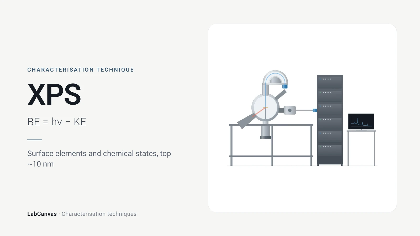
X-ray photoelectron spectroscopy (XPS, also called ESCA) shines X-rays on a sample and measures the kinetic energy of the core electrons they eject; from the photon energy and that kinetic energy the electron’s binding energy follows (Baio et al. 2020). Binding energies identify every element except hydrogen and helium, and small shifts in them reveal oxidation states and bonding (Baio et al. 2020). Because the photoelectrons escape only from the outermost few nanometres, about 2–10 nm, XPS is a surface technique that gives quantitative surface composition and chemistry (Baio et al. 2020).
Contents
X-ray photoelectron spectroscopy (XPS) at a glance
| Probe | Monochromatic Al Kα X-rays, 1487 eV, in most laboratory instruments (Baio et al. 2020); Mg Kα, 1253.6 eV, is also used (Shulga et al. 2021) |
|---|---|
| Signal measured | Kinetic energy of photoelectrons, converted to binding energy through the photon energy (Baio et al. 2020) |
| Main information | Elemental composition and chemical (oxidation) states of the surface region (Baio et al. 2020) |
| Elements detected | All except H and He (Baio et al. 2020); lithium to uranium (Kuzmyn et al. 2026) |
| Sampling depth | 2–10 nm (Baio et al. 2020); taken as 3λ, the depth from which 95% of photoelectrons come, 3–10 nm for Al Kα (Susi et al. 2015) |
| Detection limit | Roughly 0.1–1 at% for elements such as Br, S, P, Si and metals (Kuzmyn et al. 2026) |
| Survey scan | Typically 0–1100 eV binding energy, to find which elements are present (Baio et al. 2020) |
| High-resolution scan | Narrow scan of one core level, e.g. C 1s, to resolve chemical species (Baio et al. 2020) |
| Chemical shift | Electronegative neighbours raise the binding energy: C 1s rises in the order C–C < C–O < C=O (Baio et al. 2020) |
| Charge referencing | C–C/C–H component set to 285.0 eV, with 284.8–285.0 eV widely used; an approximate correction, not an absolute calibration (Kuzmyn et al. 2026) |
| Quantification | Peak areas divided by relative sensitivity factors, then normalised to 100% (Kuzmyn et al. 2026) |
| Environment | Ultra-high vacuum; samples must be vacuum compatible (Baio et al. 2020) |
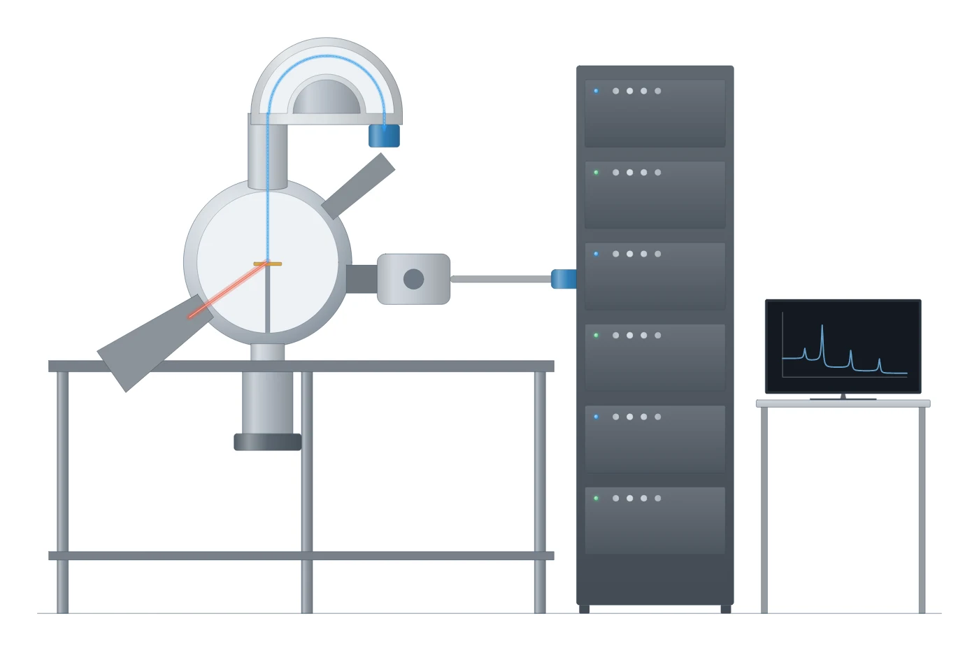
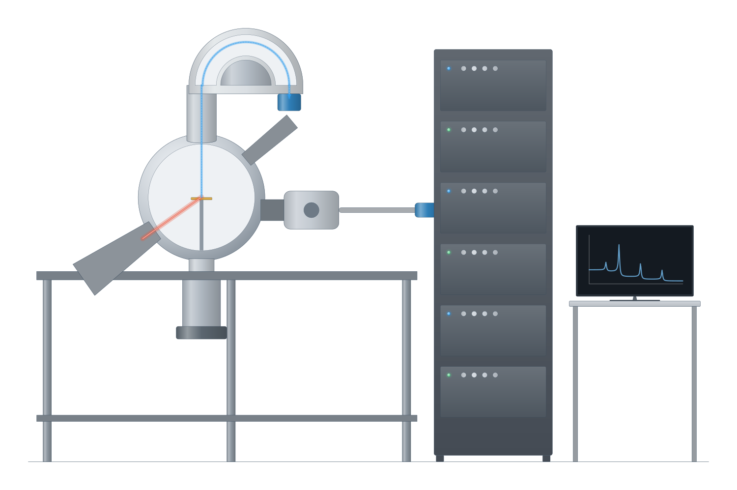
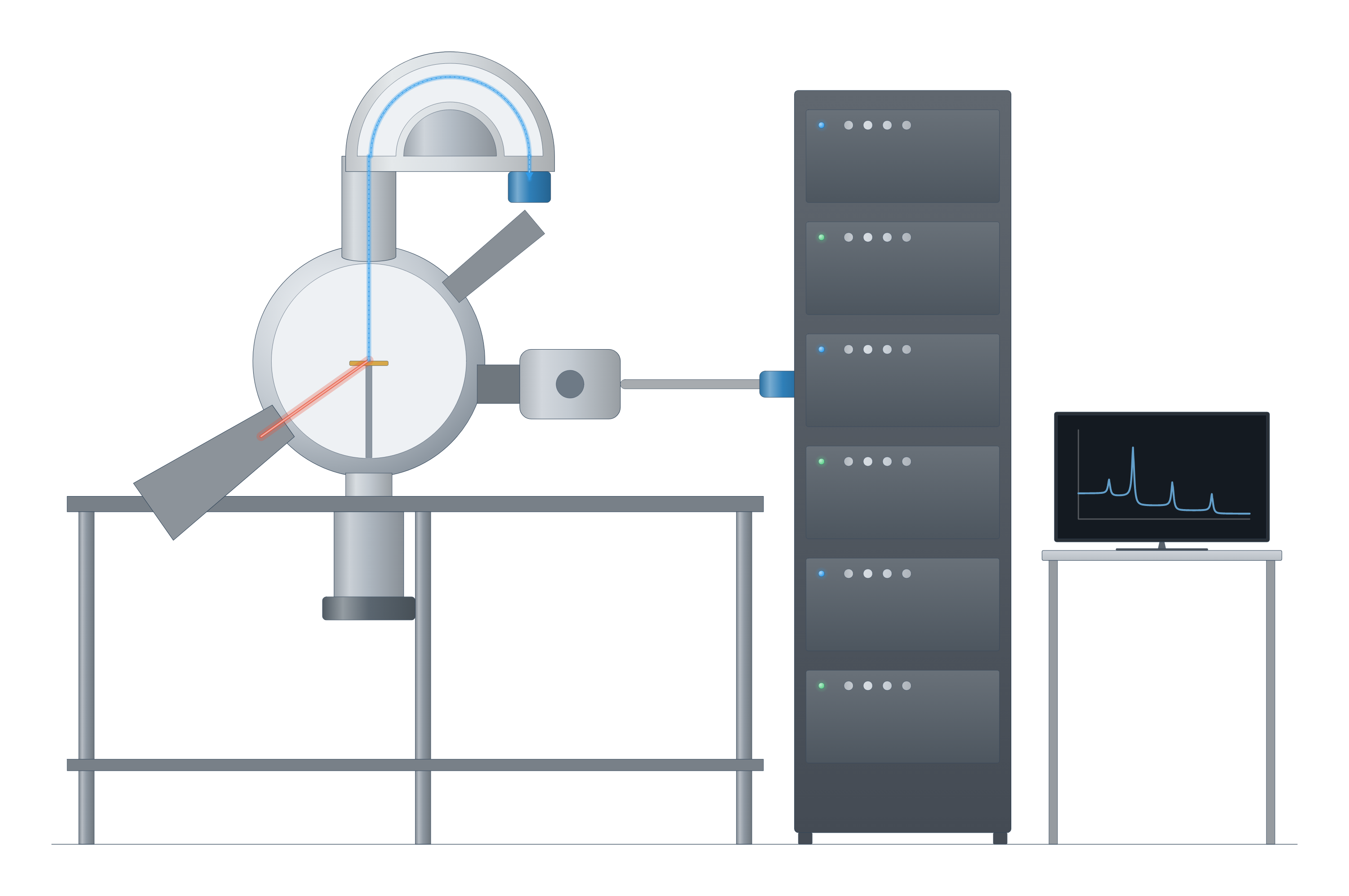
X-ray photoelectron spectroscopy (XPS) instrument drawing (high-resolution SVG)
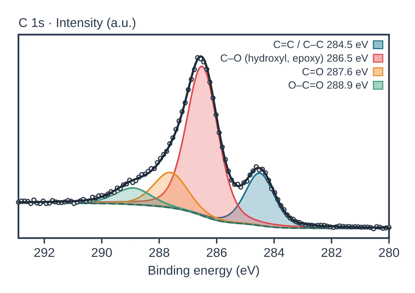
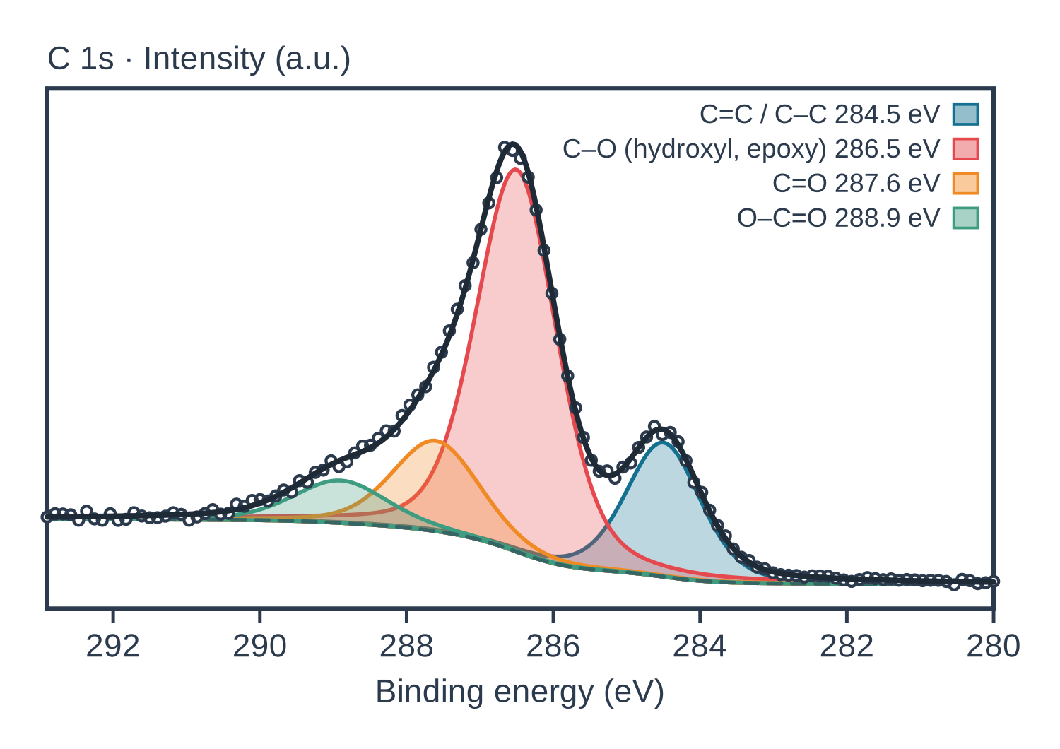
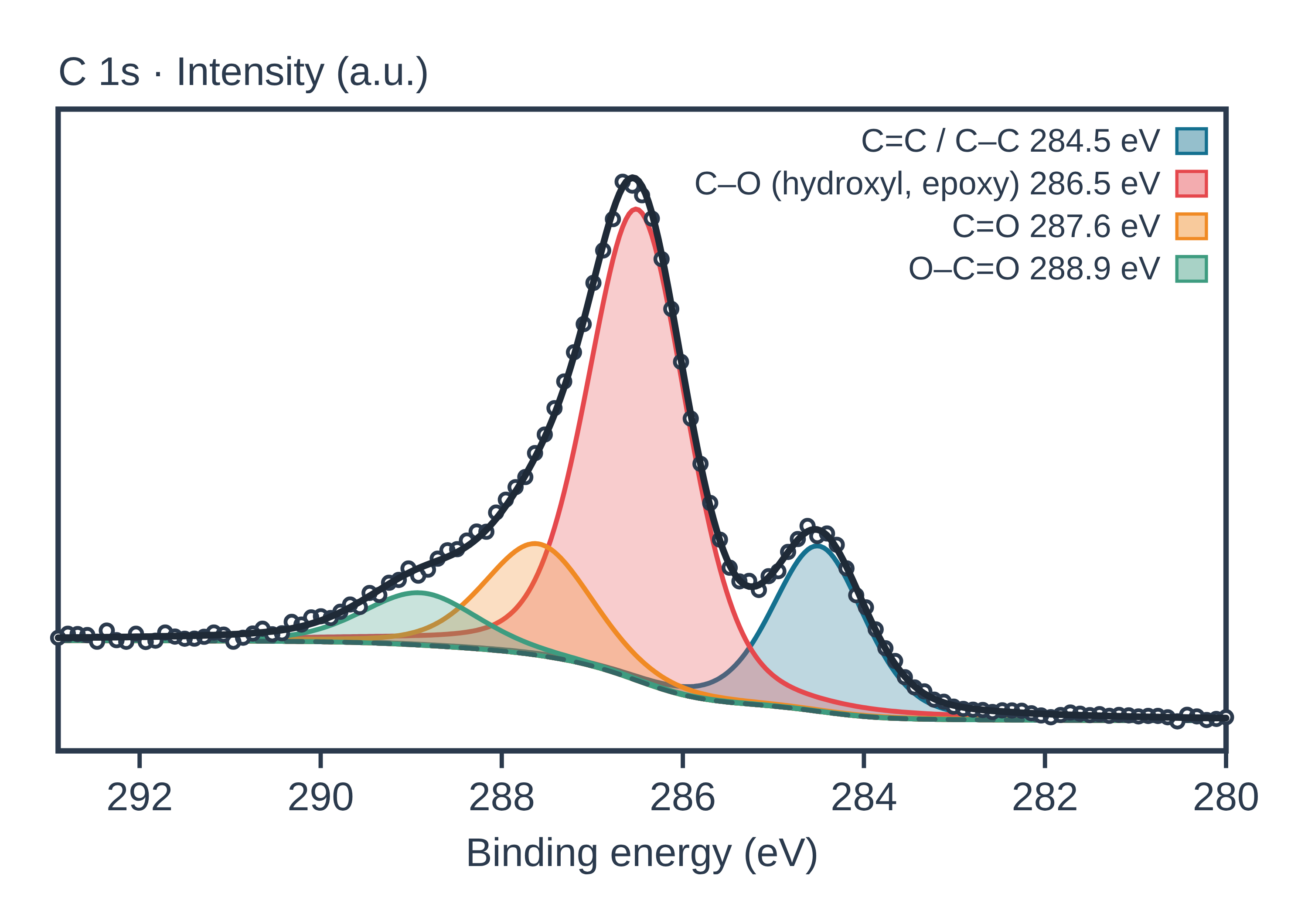
X-ray photoelectron spectroscopy (XPS) data: an example plot to edit
How XPS works
XPS is based on the photoelectric effect. An X-ray photon of energy hν is absorbed by an atom and ejects a core electron; if hν exceeds the electron’s binding energy, the photoelectron leaves with a measurable kinetic energy. The Einstein equation links the three quantities, so measuring the kinetic energy with an electron analyser and knowing the photon energy gives the binding energy: BE = hν − KE (Baio et al. 2020). The most common laboratory source is monochromatic Al Kα at 1487 eV (Baio et al. 2020).
Each element has core levels at characteristic binding energies, so peak positions identify the elements present; all elements except hydrogen and helium are detected (Baio et al. 2020). The exact energy of a peak also depends on the atom’s chemical environment, which is what makes XPS a chemical-state technique.
Why it is surface sensitive. The X-rays penetrate microns into the sample, but the photoelectrons have kinetic energies of a few hundred eV and interact strongly with matter, so only those from near the surface escape without losing energy. The sampling depth is about 2–10 nm, depending on the emission angle and the material (Baio et al. 2020). It is usually taken as three inelastic mean free paths, the depth from which 95% of the photoelectrons come: 3–10 nm for Al Kα, and 8.7 nm, about 26 graphene layers, for graphite (Susi et al. 2015).
What the data looks like and how to read it
XPS spectra are plotted as counts against binding energy, with binding energy increasing from right to left (Baio et al. 2020).
- Survey (wide) scan. A scan over about 0–1100 eV shows which elements are present and how much of each; peak areas, corrected for the probability of creating and detecting each photoelectron, give the composition (Baio et al. 2020). Atomic percentages come from areas divided by relative sensitivity factors, never from raw peak areas (Kuzmyn et al. 2026).
- High-resolution (narrow) scans. A narrow scan of one core level, such as C 1s, resolves chemical species. Bonding carbon to more electronegative atoms raises its binding energy, so C 1s increases in the order C–C < C–O < C=O (Baio et al. 2020). In a poly(2-hydroxypropyl methacrylamide) brush, for example, C–C/C–H, C–N, C–O and C=O components appeared near 285.0, 286.1, 287.0 and 288.0 eV in the ratio expected from the repeat unit (Kuzmyn et al. 2026).
- Background. Inelastically scattered electrons add a stepped background on the high-binding-energy side of each peak; it is removed with a linear, Shirley or Tougaard background before fitting (Susi et al. 2015).
- Line shapes. Peaks are usually fitted with Voigt (Gaussian–Lorentzian) profiles; metallic systems such as graphite give an asymmetric Doniach–Šunjić C 1s line, with the graphite maximum at 284.42 eV (Susi et al. 2015).
- Doublets. Spin–orbit coupling splits levels such as P 2p into two components; for P 2p the predicted splitting is 0.87 eV, with the lower-binding-energy 2p₃/₂ component twice the area of 2p₁/₂ (Susi et al. 2015).
The background shape also hints at depth: atoms at the outermost surface give a background that rises little above the peak, while atoms buried deeper give a steadily rising background (Baio et al. 2020).
Sample preparation
- Keep the surface clean. Any solvent exposure, even rinsing, can deposit contaminants and change the surface composition; plan sample handling as part of the experiment (Baio et al. 2020).
- Make it vacuum compatible. XPS runs in ultra-high vacuum, so samples must not outgas, and moving a sample from water into vacuum can rearrange its surface. Frozen-hydrated preparation can lock in a hydrated surface structure (Baio et al. 2020).
- Powders can be pressed into small cups; freeze-dried microbial cells, for example, form powders that are pressed and analysed this way (Wei et al. 2021).
- Control charging. Insulating samples charge positively during analysis, which shifts and broadens peaks; low-energy electron flood guns or dual-mode neutralisers compensate, and their settings should be reported (Kuzmyn et al. 2026).
- Watch for beam damage. Measure sensitive regions early, take several short scans and compare the first and last for changes in area, position or width (Kuzmyn et al. 2026).
Charge referencing and depth profiling
Charge referencing to C 1s. On insulators the binding-energy scale is usually corrected by setting the lowest-energy C 1s component, from C–C/C–H carbon, to 285.0 eV; values from 284.8 to 285.0 eV are widely used (Kuzmyn et al. 2026). Treat this as an approximate correction: adventitious carbon is an unreliable reference because its apparent energy varies with substrate, surface condition and charging; a visible conductive substrate peak such as Au 4f or Si 2p can be a better reference; differential charging cannot be fixed by one rigid shift; and forcing C 1s to 285.0 eV can hide real chemical shifts. Report both raw and corrected binding energies when small shifts matter (Kuzmyn et al. 2026). For carbon nanomaterials, the C 1s position must be measured for each sample rather than assumed as a common reference, and the energy scale calibrated with a clean metal (Susi et al. 2015).
Depth profiling. Because the XPS signal decays exponentially with depth, a spectrum is a weighted average over the sampling depth, and extracting a composition profile from it alone needs modelling (Baio et al. 2020). Alternatively, the surface is removed step by step with an ion beam between measurements. For organic layers, argon gas cluster ion beams with about 500–2000 atoms per cluster are preferred, because monatomic Ar⁺ sputtering causes cross-linking, carbonisation and preferential sputtering; X-ray exposure itself can change sputter rates in some polymers (Kuzmyn et al. 2026). Thickness of thin coatings can also be estimated from how much they attenuate the substrate signal (Kuzmyn et al. 2026), and varying the excitation energy, including hard X-rays, probes coatings on core–shell nanoparticles (Radnik et al. 2022).
What XPS tells you about materials
Doped graphene and carbon. XPS is one of the main tools for the concentration and bonding of nitrogen, boron and phosphorus dopants in graphene and carbon nanotubes (Susi et al. 2015). In N 1s spectra, a component near 398.3 ± 0.3 eV is commonly assigned to pyridinic nitrogen and one near 400.1 ± 0.3 eV to pyrrolic nitrogen, while values from about 400.2 to 401.8 eV have been assigned to substitutional (graphitic) nitrogen; the spread is large, so assignments need care (Susi et al. 2015). For oxidised carbons such as those made from graphene oxide, C 1s components above about 285.1 eV are attributed to carbon bonded to oxygen (Shulga et al. 2021).
Oxide electrodes and coatings. XPS gives the elemental composition and oxidation states of solid-oxide fuel-cell cathodes to a depth of about 5–10 nm and is used to follow cation enrichment at their surfaces; changes in the surface chemical state are linked to performance degradation (Anwar et al. 2022). For composition and thickness of nanoparticle coatings it can be combined with modelling of peak intensities (Radnik et al. 2022).
Thin organic films. XPS sees the outermost ~10 nm of organic films, so for polymer brushes thicker than about 20 nm the elemental ratios reflect the monomer composition (Kuzmyn et al. 2026).
XPS does not tell you the crystal structure: pair it with XRD, which averages over the bulk (Abid et al. 2023). Studies of carbon materials often combine XPS with Raman spectroscopy and electron energy-loss measurements, because the techniques give different estimates of the same quantity (Shulga et al. 2021). See also FTIR and ICP-MS, and the characterisation techniques hub for how they all compare.
Common mistakes and limits
- Quantifying from raw areas. Each core level has a different photoionisation cross-section and analyser transmission; compare sensitivity-factor-corrected areas and report the factor library used (Kuzmyn et al. 2026).
- Over-fitting peaks. Assigning binding energies to specific structures is rarely straightforward, and overlapping ranges have been reported for the same configurations (Susi et al. 2015). Symmetric fit functions on an asymmetric C 1s line overestimated the sp³ carbon content of a porous carbon (Shulga et al. 2021).
- Trusting adventitious carbon blindly. Its apparent binding energy depends on the substrate and charging (Kuzmyn et al. 2026).
- Ignoring the background. A careful background subtraction is vital for analysing the primary spectrum (Susi et al. 2015), and the same model should be used for all spectra being compared (Kuzmyn et al. 2026).
- Calling XPS a bulk measurement. It reports the top few nanometres; for thin materials such as graphitic nanomaterials (8.7 nm sampling depth in graphite) it can in effect probe the whole thickness (Susi et al. 2015).
- Overlooking contamination. Some contaminants are easier to see by other methods: ToF-SIMS is far more sensitive to PDMS than XPS (Baio et al. 2020).
How to draw the XPS setup and data in LabCanvas
A clear XPS methods figure shows the X-ray source, the sample in vacuum, the electron energy analyser and the detector, with the photoelectron path from the surface to the analyser. In LabCanvas the figure editor’s Library has the XPS instrument as an editable object, including a cutaway of the X-ray and photoelectron paths, and an editable data plot for survey and high-resolution spectra. You can reverse the binding-energy axis, label core-level peaks (C 1s, O 1s, N 1s), add fitted components with their assignments and export the figure for a methods section or graphical abstract.
XPS compared with other surface techniques
| Technique | What it measures | Sampling depth | Notes | Source |
|---|---|---|---|---|
| XPS | Elemental composition (all but H, He) and chemical states | 2–10 nm | Quantitative; ultra-high vacuum | Baio et al. 2020 |
| ToF-SIMS | Mass spectra of ions sputtered from the surface; molecular structure | About 2 nm in low-dose mode | Very sensitive (e.g. to PDMS); quantification difficult | Baio et al. 2020 |
| NEXAFS | Core-level absorption: chemical bonds and their orientation | 1–10 nm for most biological materials | Needs synchrotron light | Baio et al. 2020 |
Related techniques
X-ray diffraction (XRD)
X-ray diffraction explained: Bragg’s law, how to read an XRD pattern, phase identification, Scherrer crystallite size, Rietveld refinement and common mistakes.
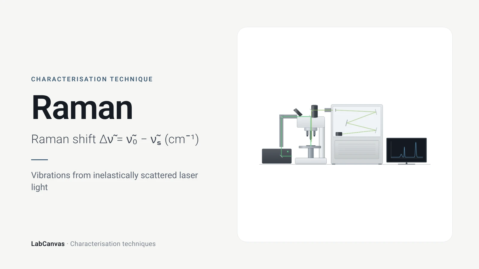
Raman spectroscopy
Raman spectroscopy explained: inelastic laser scattering, Raman shift, Stokes lines, IR complementarity, graphene D, G and 2D bands, lasers, fluorescence.
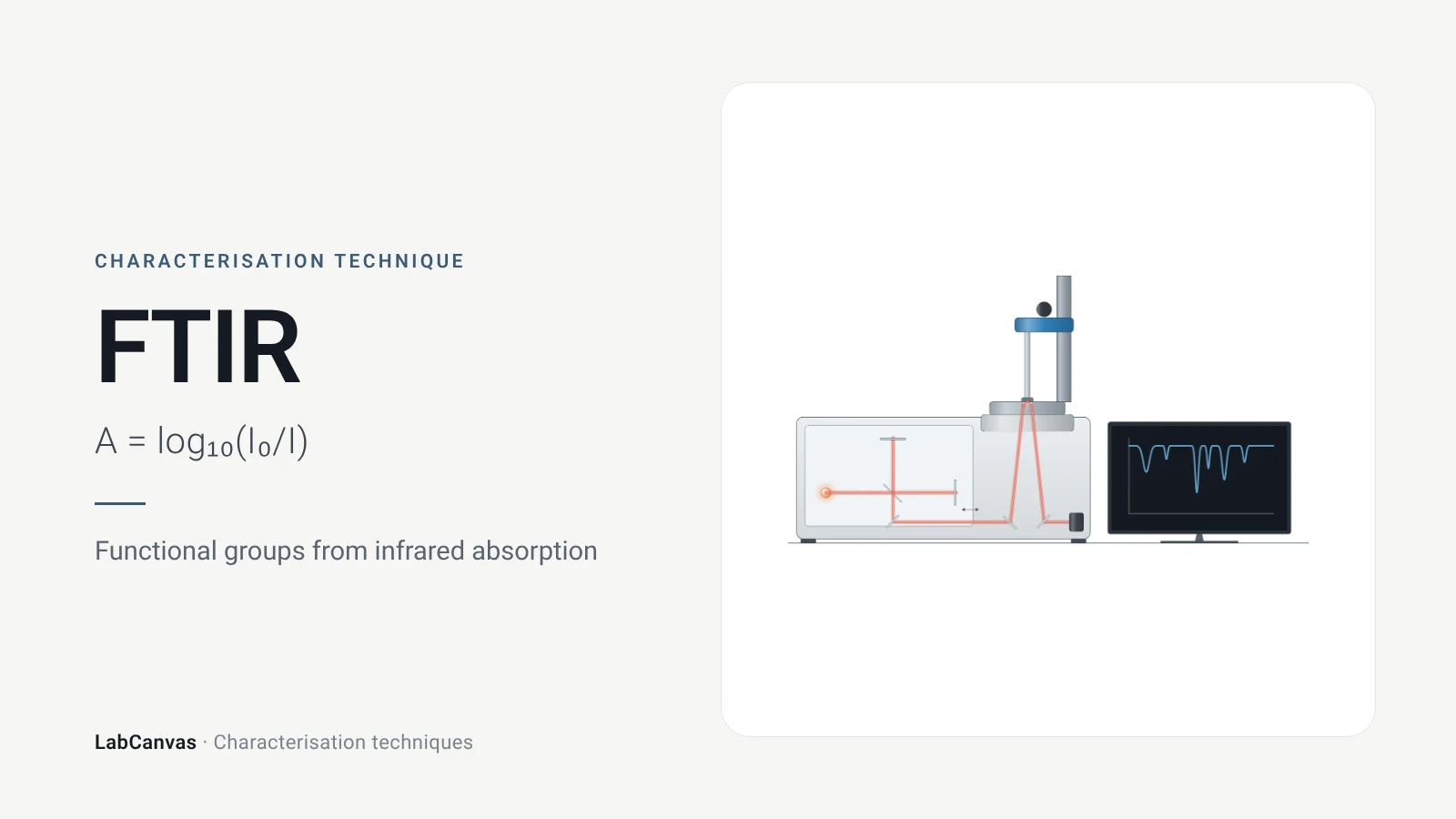
Fourier-transform infrared (FTIR) spectroscopy
FTIR spectroscopy explained: infrared absorption by bond vibrations, the interferometer and Fourier transform, wavenumber regions, ATR and reading bands.
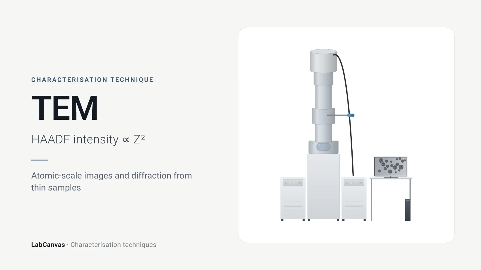
Transmission electron microscopy (TEM)
How TEM works: bright field, HRTEM lattice images, SAED diffraction, STEM-HAADF Z-contrast, EDS/EELS, sample thickness and beam damage of MOFs.
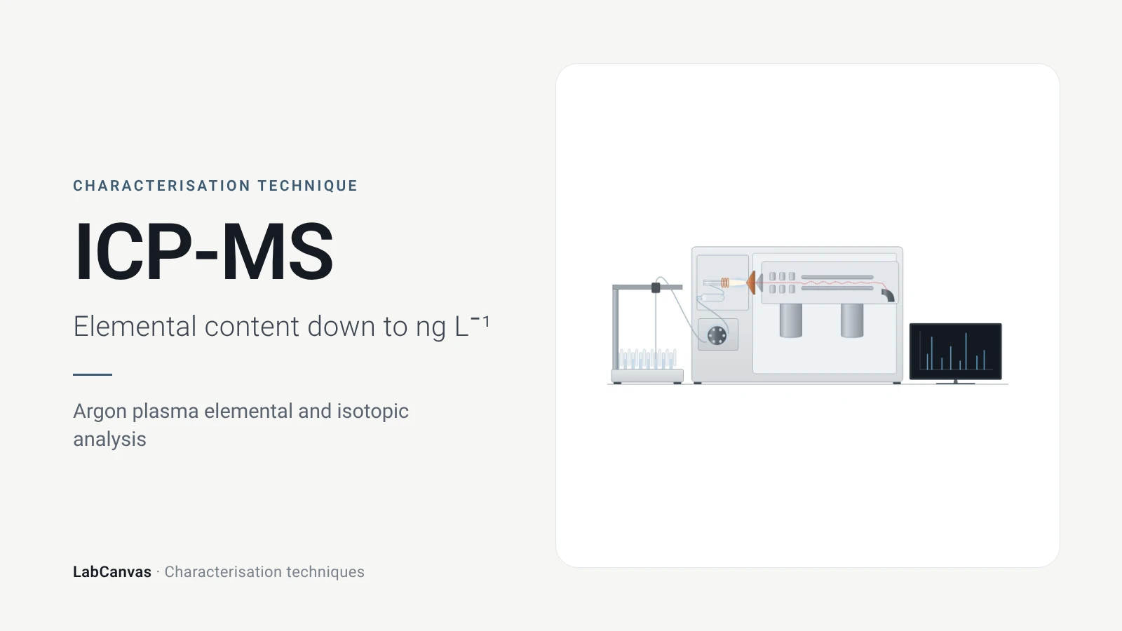
ICP-MS and ICP-OES
ICP-MS and ICP-OES explained: argon plasma, detection limits, acid digestion, interferences, single-particle ICP-MS and metal content of MOFs.
More on LabCanvas
- All characterisation techniques: XRD, XPS, BET, SEM, TEM, NMR, FTIR, Raman and more, explained with cited sources
- Graphical abstract sizes and templates: ACS, Wiley, Angewandte, RSC, Elsevier and Cell Press, with templates at the right size
- Materials explained: MOFs, COFs, 2D materials, perovskites, batteries and zeolites, with cited facts
- Journal figure size guide: Column widths and resolutions for 38 journals
Frequently asked questions
What is XPS used for?
XPS measures which elements are present at a surface, in what amounts and in what chemical states, for polymers, metals, ceramics and biological materials, as powders, films, particles or fibres (Baio et al. 2020).
How does XPS work?
X-rays eject core electrons from atoms in the sample; an analyser measures their kinetic energy, and the binding energy follows from the photon energy minus that kinetic energy (Einstein equation). Binding energies identify elements and chemical states (Baio et al. 2020).
How deep does XPS analyse?
About 2–10 nm, depending on the material and emission angle (Baio et al. 2020). The sampling depth is usually taken as three inelastic mean free paths, 3–10 nm for Al Kα X-rays (Susi et al. 2015).
What is the difference between a survey scan and a high-resolution scan in XPS?
A survey scan covers about 0–1100 eV and shows which elements are present and their amounts; a high-resolution scan covers one core level, such as C 1s, at higher energy resolution to separate chemical species (Baio et al. 2020).
How do you charge-correct XPS spectra?
For insulating samples, the C–C/C–H component of C 1s is commonly set to 285.0 eV, with 284.8–285.0 eV widely used. This is only approximate; a conductive substrate peak can be a better reference, and raw and corrected values should both be reported (Kuzmyn et al. 2026).
Why can XPS not detect hydrogen?
The cross-sections for ejecting photoelectrons from hydrogen and helium are too low for them to be detected, so XPS sees all elements except H and He (Baio et al. 2020).
How is XPS depth profiling done?
The surface is sputtered away with an ion beam between measurements. For organic materials argon gas cluster ion beams are preferred because monatomic Ar⁺ damages the chemistry by cross-linking and carbonisation (Kuzmyn et al. 2026).
XPS vs XRD: what is the difference?
XPS gives elemental composition and chemical states of the top 2–10 nm (Baio et al. 2020); XRD gives the crystal structure and phases of the bulk, averaged over all crystallites in the beam (Abid et al. 2023).
References
- J. E. Baio, D. J. Graham, D. G. Castner. Surface analysis tools for characterizing biological materials. Chem. Soc. Rev. 2020, 49, 3278–3296. doi:10.1039/d0cs00181c
- T. Susi, T. Pichler, P. Ayala. X-ray photoelectron spectroscopy of graphitic carbon nanomaterials doped with heteroatoms. Beilstein J. Nanotechnol. 2015, 6, 177–192. doi:10.3762/bjnano.6.17
- A. R. Kuzmyn, G.-J. Linker, Y. Bu, S. de Beer. XPS analysis of polymer brush coatings. Polym. Chem. 2026, 17, 3731–3745. doi:10.1039/d6py00562d
- M. Anwar, M. A. Shaikh Abdul, U. M. Khan, M. Hassan, A. H. Khoja, A. Muchtar. A review of X-ray photoelectron spectroscopy technique to analyze the stability and degradation mechanism of solid oxide fuel cell cathode materials. Materials 2022, 15, 2540. doi:10.3390/ma15072540
- J. Radnik et al.. Composition, thickness, and homogeneity of the coating of core-shell nanoparticles: possibilities, limits, and challenges of X-ray photoelectron spectroscopy. Anal. Bioanal. Chem. 2022, 414, 4331–4345. doi:10.1007/s00216-022-04057-9
- H. Wei, X.-Y. Yang, H. C. van der Mei, H. J. Busscher. X-ray photoelectron spectroscopy on microbial cell surfaces: a forgotten method for the characterization of microorganisms encapsulated with surface-engineered shells. Front. Chem. 2021, 9, 666159. doi:10.3389/fchem.2021.666159
- Y. M. Shulga et al.. The concentration of C(sp³) atoms and properties of an activated carbon with over 3000 m²/g BET surface area. Nanomaterials 2021, 11, 1324. doi:10.3390/nano11051324
- H. R. Abid, M. R. Azhar, S. Iglauer, Z. H. Rada, A. Al-Yaseri, A. Keshavarz. Physiochemical characterization of metal organic framework materials: a mini review. Heliyon 2023, 10, e23840. doi:10.1016/j.heliyon.2023.e23840
Draw X-ray photoelectron spectroscopy (XPS) figures for your paper
LabCanvas is a browser workspace for scientific figures: instruments with their beam and light paths, editable data plots, crystal structures, graphs and graphical abstracts at journal sizes.
Draw X-ray photoelectron spectroscopy (XPS) in LabCanvas