Materials characterisation techniques: what each one measures and when to use it

Materials characterisation is the set of measurements that tell a chemist what a new material is: its crystal structure (XRD, which identifies phases from Bragg diffraction; Abid et al. 2023), its surface chemistry (XPS, which reads the top 2–10 nm; Baio et al. 2020), its porosity (gas sorption and the BET surface area; Osterrieth et al. 2022), its size and shape (SEM, TEM, AFM and DLS), its bonding (NMR, FTIR and Raman), its stability (TGA and DSC), its optical band gap (UV–vis), its composition (ICP-MS) and its electrochemistry (cyclic voltammetry and EIS). No single technique is enough; each page below explains how one method works, what its data looks like, how to prepare samples and the mistakes to avoid, with every fact cited.

Characterisation techniquesPublished 27 October 2026Last updated 27 October 202627 references

Characterisation techniques: How materials chemists measure structure, surface and composition (XRD · XPS · BET · SEM · TEM · NMR)

Contents

Characterisation techniques at a glance

Characterisation techniques: key facts, with sources
Crystal structure	XRD: Bragg’s law nλ = 2d sin θ gives peak positions that fingerprint the phase (Wang et al. 2026; Abid et al. 2023)
Surface composition	XPS: all elements except H and He, from the top 2–10 nm (Baio et al. 2020)
Porosity	Gas sorption with N₂ at 77 K; the BET method is the most widely used surface-area metric (Abid et al. 2023; Osterrieth et al. 2022)
Morphology	SEM: secondary electrons show topography, backscattered electrons atomic-number contrast (Erlich et al. 2020)
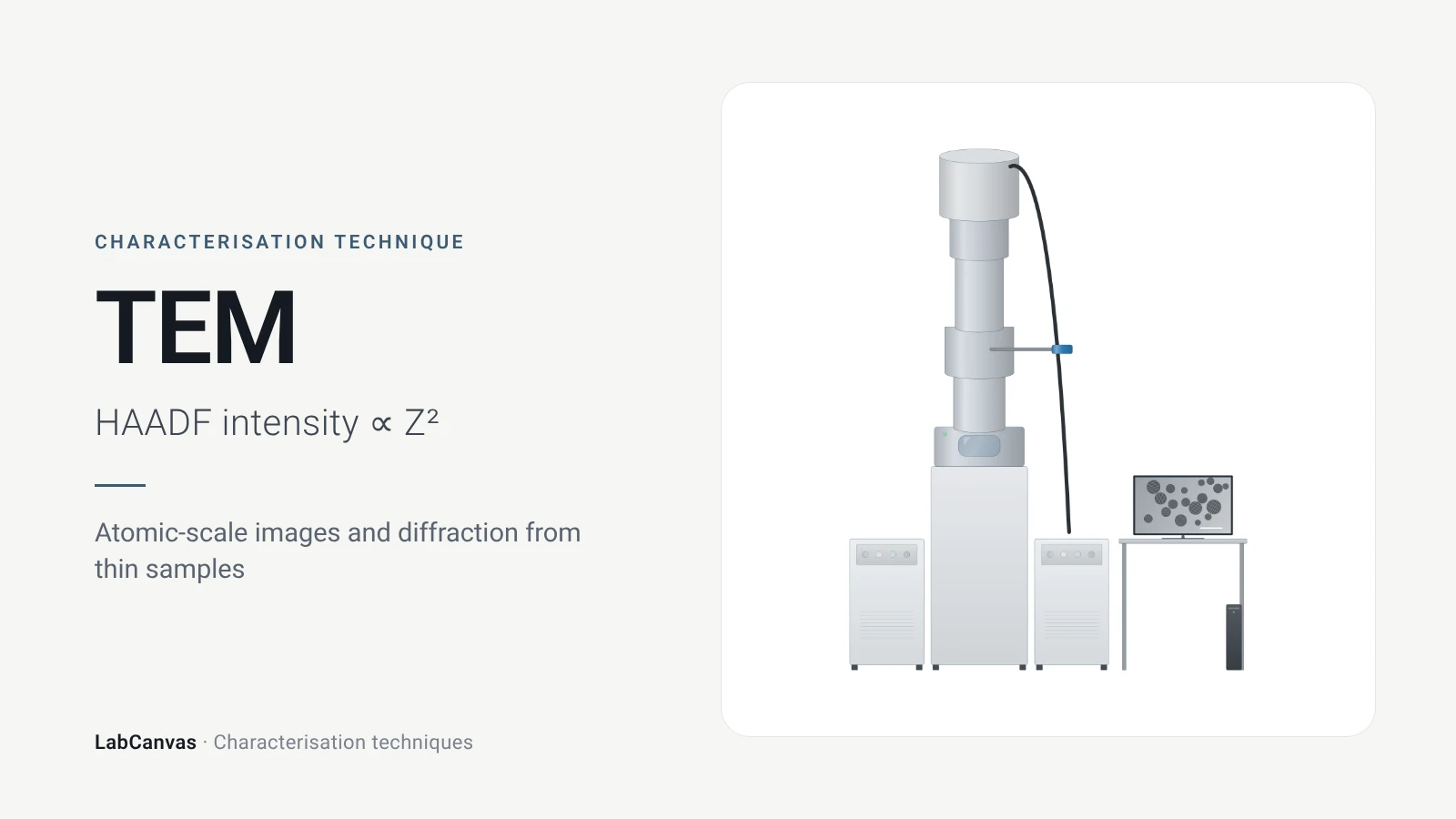
Atomic-scale imaging	TEM: samples below about 100 nm thick; HAADF-STEM intensity roughly ∝ Z² (Bijelić et al. 2023)
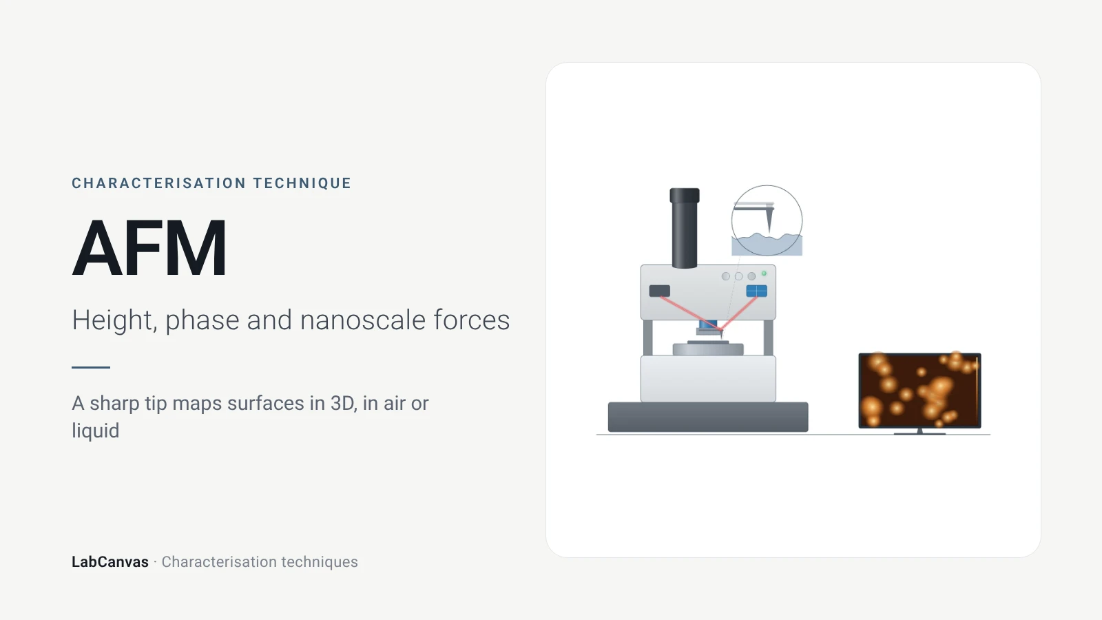
Height and roughness	AFM: 1–10 nm lateral and sub-nanometre vertical resolution, no vacuum (Joo et al. 2025)
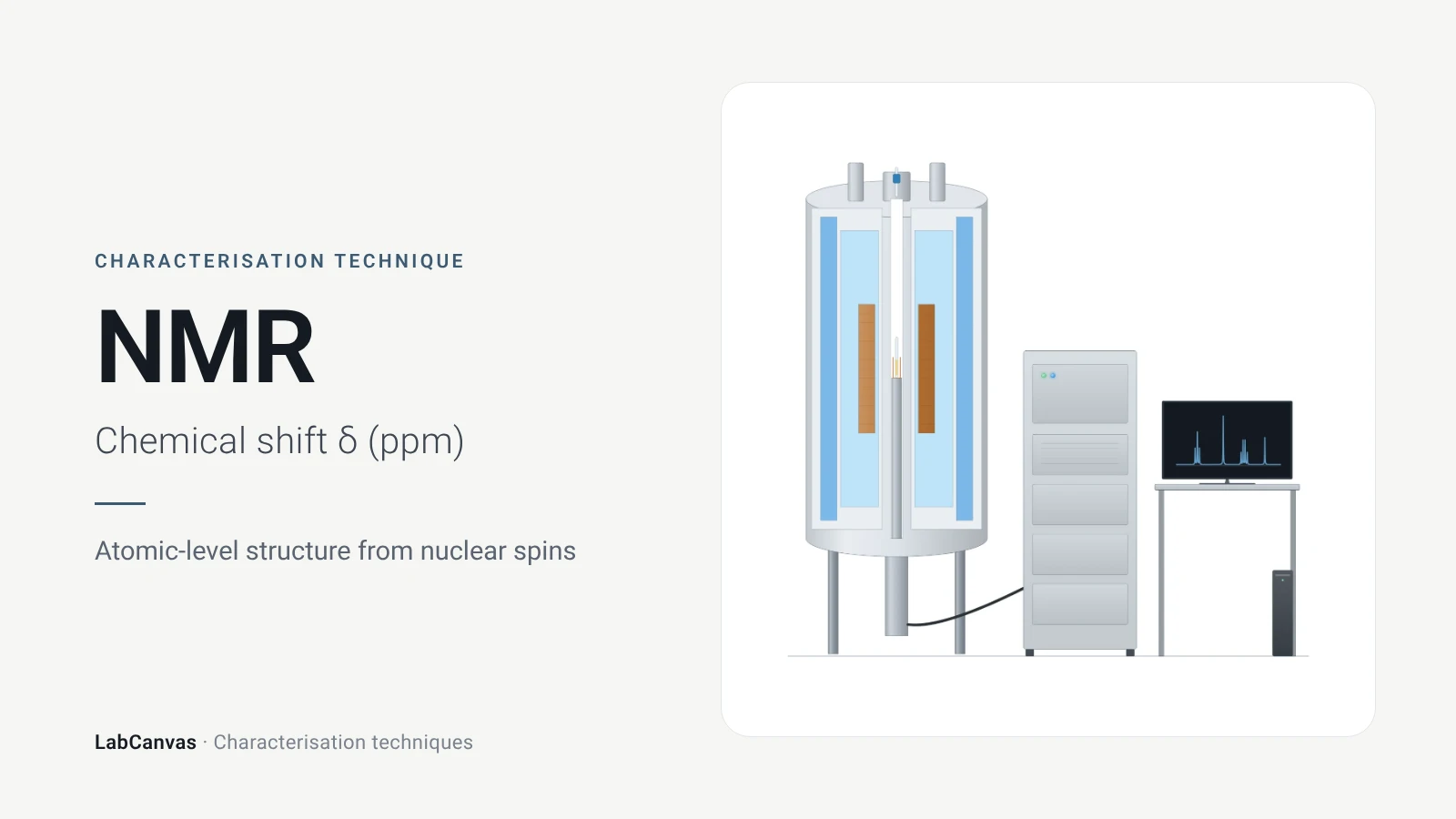
Local structure and bonding	NMR chemical shifts (Armitage et al. 2013); solid-state MAS NMR for MOFs and zeolites (Brunner & Rauche 2020)
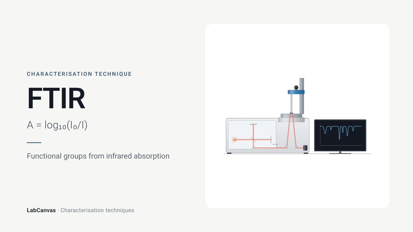
Vibrational spectra	FTIR needs a dipole change (Baker et al. 2014); Raman needs a polarisability change (Jones et al. 2019)
Thermal stability	TGA records mass against temperature; DSC records heat flow (Abid et al. 2023; Leyva-Porras et al. 2019)
Band gap	UV–vis with a Tauc plot; diffuse reflectance for powders (Escobedo-Morales et al. 2019)
Size in liquid	DLS gives the hydrodynamic diameter through the Stokes–Einstein equation (Wishard & Gibb 2019)
Elemental composition	ICP-MS: more than 65 elements, ng L⁻¹ detection limits for most (Mazarakioti et al. 2022)
Electrochemistry	Cyclic voltammetry (Rafiee et al. 2024) and impedance spectroscopy (Lazanas & Prodromidis 2023)

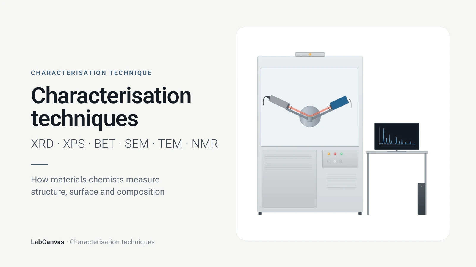
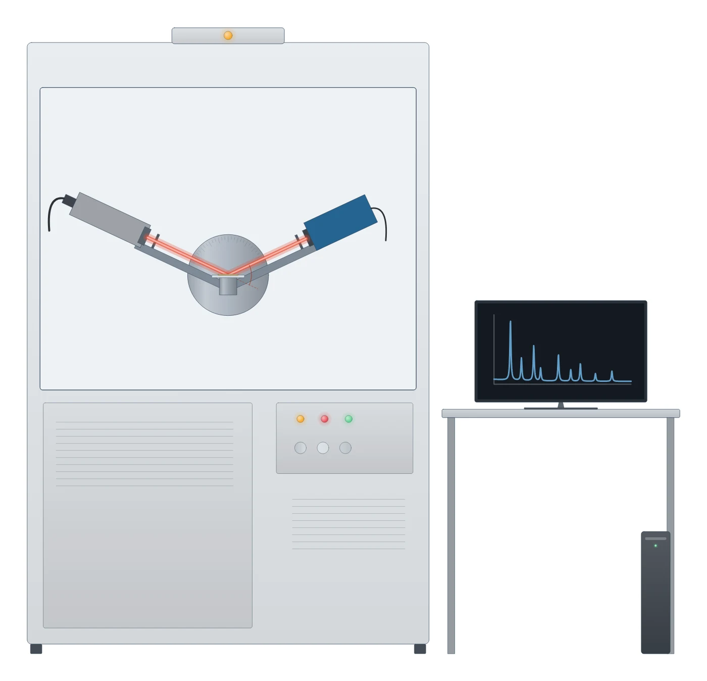
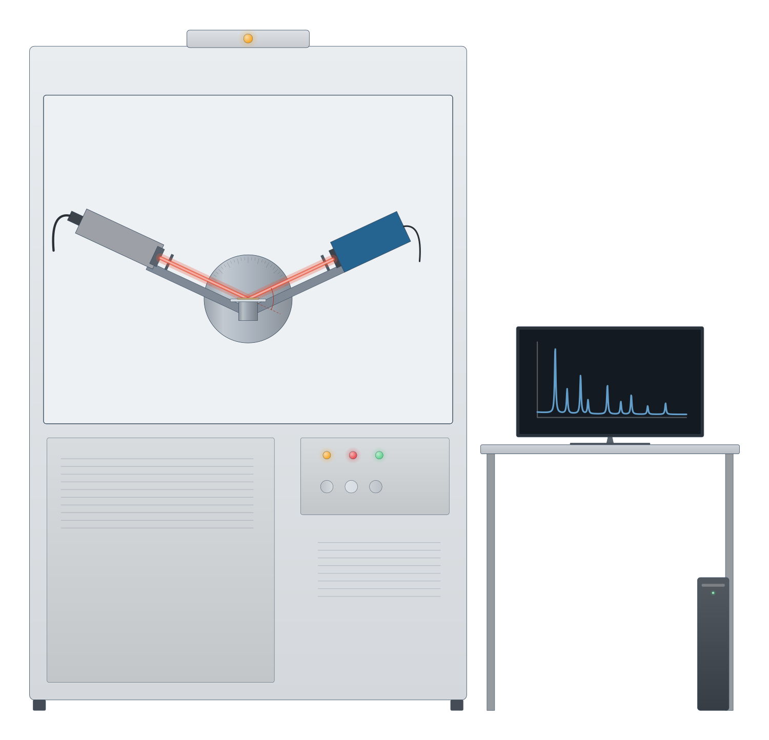
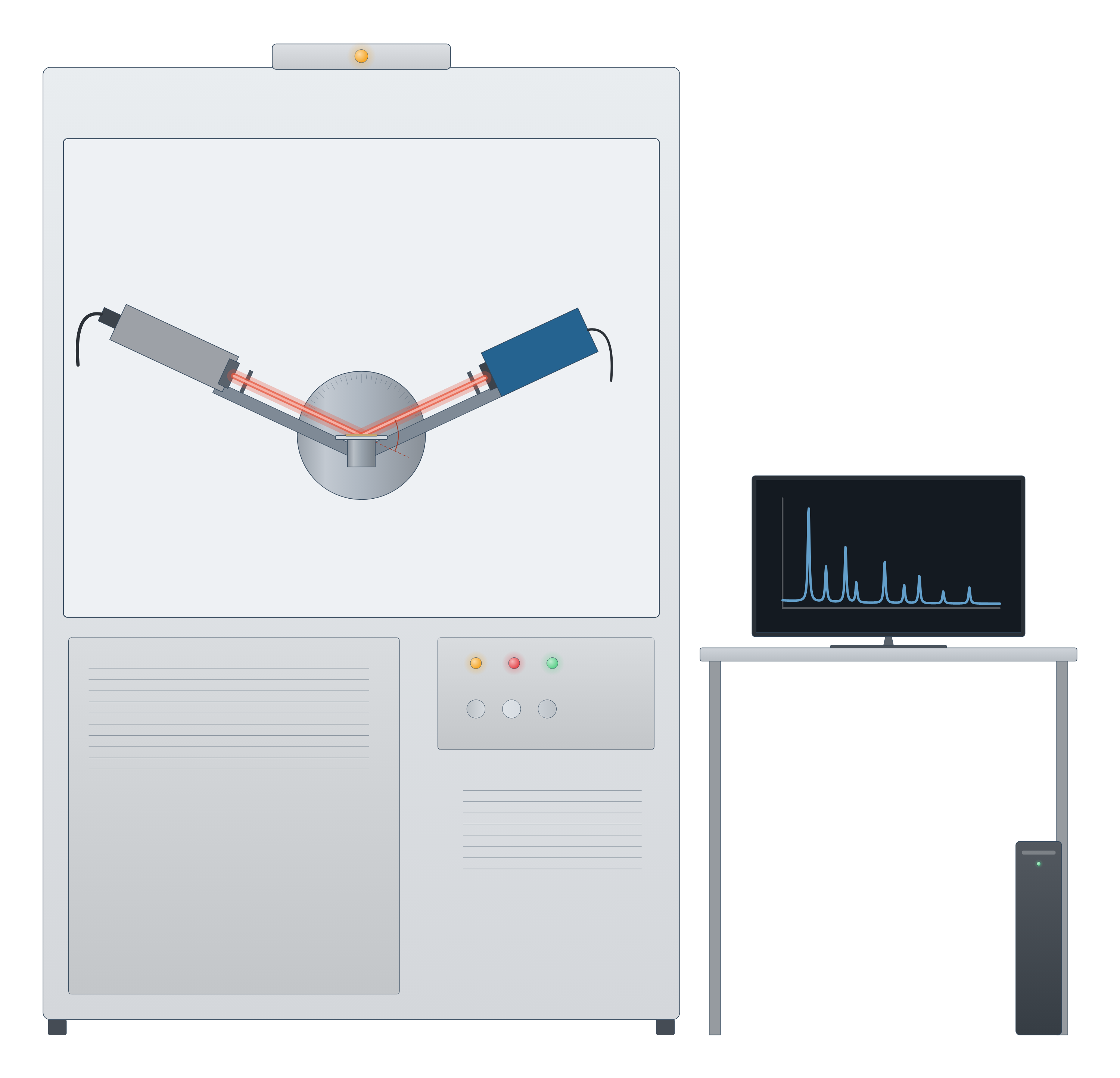
Characterisation technique instrument drawing (high-resolution SVG)

Characterisation techniques instrument drawn as a LabCanvas Library object — An X-ray diffractometer, the first instrument most new materials meet, as a LabCanvas Library drawing. Every technique page has its own instrument drawing and an example data plot to edit in the figure editor.

Edit the drawing in LabCanvas Download SVG Download PNG (3000 px)

Which characterisation technique do I need?

Start from the question, not the instrument. A typical new solid, a MOF, a nanoparticle batch or a battery cathode, goes through several of these in turn:

Is it the phase I meant to make? X-ray diffraction. Peak positions are set by the unit cell, so the pattern is compared with a simulated or published one; it is the first check on a new MOF (Abid et al. 2023).
What does it look like? SEM for particle size, shape and morphology over large areas (Erlich et al. 2020); TEM for lattice fringes, defects and particles a few nanometres across (Bijelić et al. 2023); AFM for true heights, such as the thickness of a 2D flake (Joo et al. 2025).
Is it porous, and how much? Gas sorption and the BET surface area, with the pressure range checked against consistency criteria for microporous solids (Gómez-Gualdrón et al. 2016; Osterrieth et al. 2022).
What is on the surface, and in what oxidation state? XPS (Baio et al. 2020).
Which bonds and groups are there? FTIR and Raman, which follow different selection rules and so complement each other (Jones et al. 2019), and NMR for atom-by-atom local structure (Armitage et al. 2013).
How stable is it, and what solvent is still inside? TGA and DSC (Abid et al. 2023; Leyva-Porras et al. 2019).
What is its band gap or colour? UV–vis (Escobedo-Morales et al. 2019).
How big are the particles in liquid, and will they stay dispersed? DLS and zeta potential (Rodriguez-Loya et al. 2023).
How much of each element, such as a metal loading? ICP-MS or ICP-OES after digestion (Mazarakioti et al. 2022).
How does it behave in a cell or as a catalyst? Cyclic voltammetry and impedance spectroscopy (Rafiee et al. 2024; Lazanas & Prodromidis 2023).

Bulk or surface, average or local

The most common mistake is to treat one measurement as the whole story. Techniques differ in where they look and how much of the sample they average:

Surface versus bulk. XPS sees only the outermost 2–10 nm (Baio et al. 2020), while powder XRD averages over the whole irradiated powder (Abid et al. 2023) and ICP-MS measures the dissolved sample (Mazarakioti et al. 2022). A surface oxide or coating can dominate XPS and be invisible to XRD.
Average versus local. XRD, BET and DLS each report one number for a large population; TEM and AFM look at individual particles, so images need enough of them to be statistically meaningful (Bijelić et al. 2023).
Different sizes are different quantities. A Scherrer size from XRD is a crystallite size, not a particle size (Jeong et al. 2008), and a DLS hydrodynamic diameter is intensity-weighted towards the largest particles (Wishard & Gibb 2019), so DLS and TEM sizes often differ (Filippov et al. 2023).
Crystalline versus amorphous. XRD needs long-range order to give sharp peaks (Abid et al. 2023); solid-state NMR reports local structure whether or not the solid is ordered and complements diffraction (Brunner & Rauche 2020).

A characterisation workflow for a new MOF

Metal–organic frameworks show how the techniques fit together, because nearly every MOF paper uses the same sequence (Abid et al. 2023):

PXRD to confirm the framework formed and is phase pure.
TGA to see solvent loss and the decomposition temperature, which sets the safe activation temperature: degas below about 75% of it (Abid et al. 2023).
Activation and N₂ sorption at 77 K for the BET area and pore volume, then PXRD again to check the framework survived (Abid et al. 2023).
FTIR to confirm solvent has left the pores (Abid et al. 2023), and digestion ¹H NMR to count linkers and missing-linker defects (Nerli et al. 2025).
SEM for crystal size and shape, and low-dose TEM where atomic detail is needed, since MOFs are damaged by the beam (Zheng et al. 2023).

See it applied on the UiO-66, HKUST-1 and MOF-5 pages, and the same logic for battery materials, 2D materials, perovskites and zeolites.

How to draw characterisation figures in LabCanvas

Every technique page comes with two editable pictures: a drawing of the instrument (an X-ray diffractometer, an electron microscope column, an AFM cantilever and laser, a potentiostat with a three-electrode cell) and an example data plot, such as a PXRD pattern, an N₂ isotherm, a Raman spectrum or a Nyquist plot. Open either in the figure editor to change labels, colours and data, paste in your own measurements, and combine them with structures from the materials pages into a figure or a graphical abstract at the exact size your journal asks for.

Free calculators help with the analysis itself: the Scherrer crystallite size calculator for XRD peak widths, the Tauc plot band gap calculator for UV–vis, and the RHE converter and Tafel slope calculator for electrochemistry.

Characterisation techniques compared

Technique	What it tells you	Probe and signal	Sample	Source
XRD	Phase, purity, lattice parameters, crystallite size	X-rays; diffracted intensity vs 2θ	Powder, film or single crystal	Abid et al. 2023; Wang et al. 2026
XPS	Surface elements and oxidation states	X-rays; photoelectron kinetic energy	Solid in ultra-high vacuum; top 2–10 nm	Baio et al. 2020
Gas sorption / BET	Surface area, pore size and volume	N₂ at 77 K (also Ar, CO₂, Kr); amount adsorbed vs P/P₀	Degassed powder	Abid et al. 2023; Osterrieth et al. 2022
SEM	Morphology, particle size; composition with EDS	Electron beam; secondary and backscattered electrons, X-rays	Solid, coated if insulating	Erlich et al. 2020; Newbury & Ritchie 2015
TEM / STEM	Atomic structure, defects, diffraction, local composition	Transmitted electrons	Below about 100 nm thick	Bijelić et al. 2023
AFM	3D topography, step heights, nanoscale properties	Sharp tip on a cantilever; deflection	Flat surface, in air or liquid	Joo et al. 2025
NMR	Local structure, bonding, quantity of each site	Radio-frequency pulses on nuclear spins	Solution, or solid with MAS	Armitage et al. 2013; Brunner & Rauche 2020
FTIR	Functional groups and bonds	Infrared absorption; needs a dipole change	Solid, liquid or film; ATR needs little preparation	Baker et al. 2014
Raman	Bonds, phases; layers and defects in graphene	Laser; inelastically scattered light	Almost any; works in water	Jones et al. 2019; Ferrari et al. 2006
TGA / DSC	Stability, solvent content, transitions	Temperature ramp; mass (TGA) or heat flow (DSC)	Milligrams of solid	Abid et al. 2023; Leyva-Porras et al. 2019
UV–vis	Concentration, band gap, plasmon band	UV and visible light; absorbance or diffuse reflectance	Solution, film or powder	Mayerhöfer et al. 2019; Escobedo-Morales et al. 2019
DLS / zeta	Hydrodynamic size, PDI, colloidal stability	Laser; intensity fluctuations, electrophoretic mobility	Dilute dispersion	Wishard & Gibb 2019; Rodriguez-Loya et al. 2023
ICP-MS / OES	Elemental composition, metal loading, leaching	Argon plasma; ions by m/z or emission lines	Digested solution	Mazarakioti et al. 2022
Cyclic voltammetry	Redox potentials, reversibility, catalytic current	Potential sweep; current	Working electrode in electrolyte	Rafiee et al. 2024
EIS	Resistances, capacitance, diffusion	Small AC signal over frequency; impedance	Electrochemical cell	Lazanas & Prodromidis 2023

Related techniques

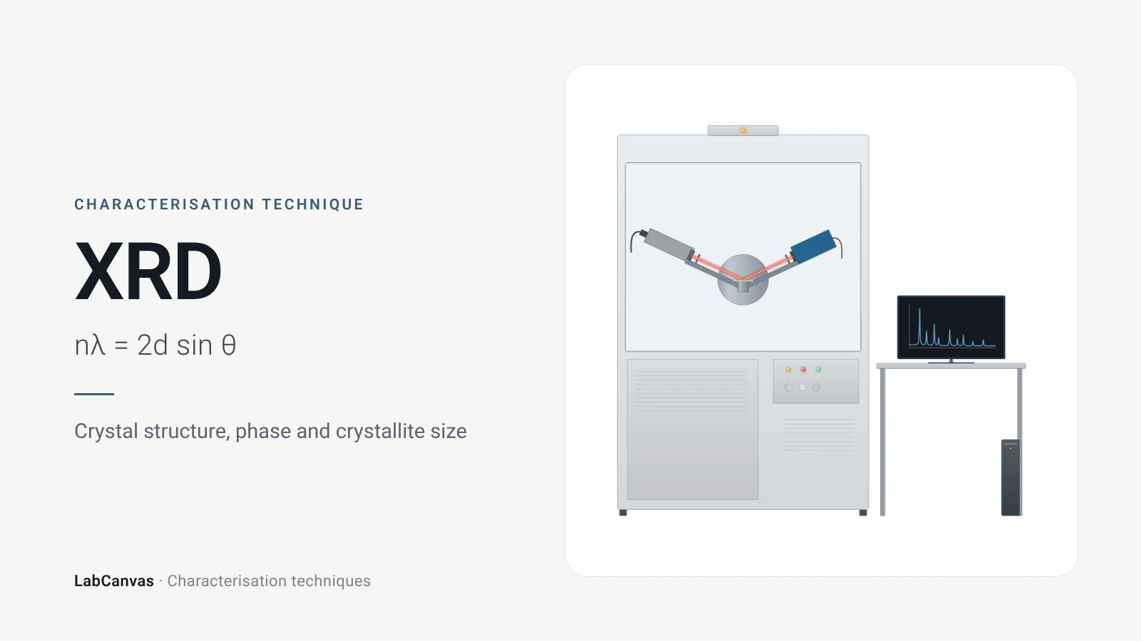
XRD: Crystal structure, phase and crystallite size (nλ = 2d sin θ)

Techniquenλ = 2d sin θ

X-ray diffraction (XRD)

X-ray diffraction explained: Bragg’s law, how to read an XRD pattern, phase identification, Scherrer crystallite size, Rietveld refinement and common mistakes.

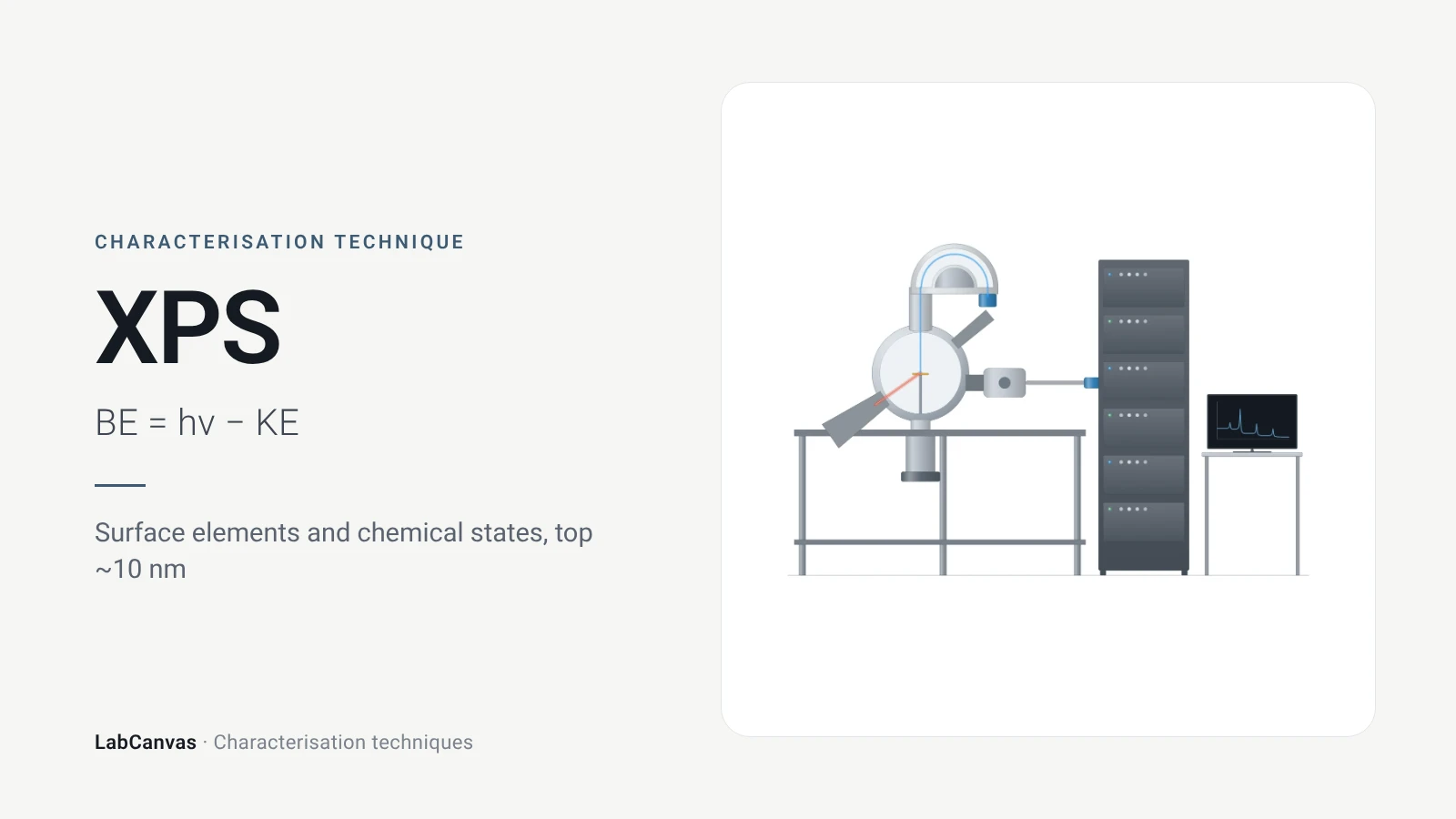
XPS: Surface elements and chemical states, top ~10 nm (BE = hν − KE)

TechniqueBE = hν − KE

X-ray photoelectron spectroscopy (XPS)

XPS explained: binding energy, 2–10 nm surface sensitivity, survey vs high-resolution spectra, chemical shifts, C 1s charge referencing and depth profiling.

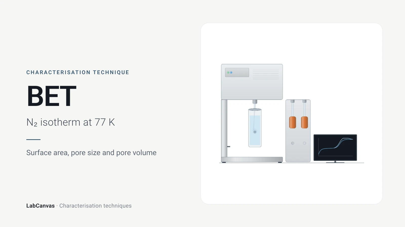
BET: Surface area, pore size and pore volume (N₂ isotherm at 77 K)

TechniqueN₂ isotherm at 77 K

Gas sorption and BET surface area

BET surface area explained: N₂ sorption at 77 K, IUPAC isotherm types, the BET range and Rouquerol criteria, pore size, degassing and limits for MOFs.

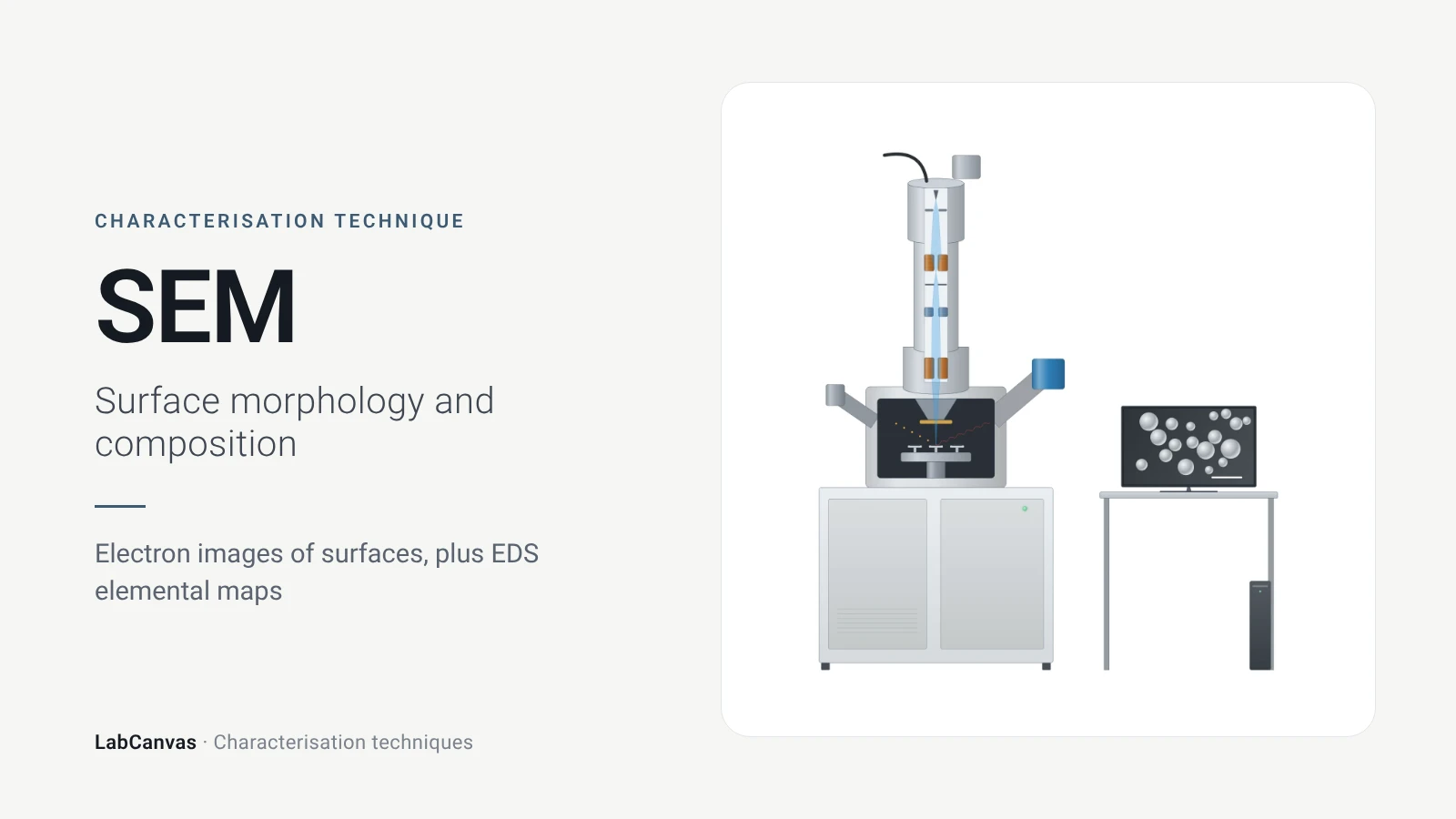
SEM: Electron images of surfaces, plus EDS elemental maps (Surface morphology and composition)

TechniqueSurface morphology and composition

Scanning electron microscopy (SEM)

How SEM works: secondary vs backscattered electron images, EDS/EDX elemental analysis, resolution, sample coating, low-vacuum mode and common mistakes.

$TEM: Atomic-scale images and diffraction from thin samples (HAADF intensity ∝ Z²)$

TechniqueHAADF intensity ∝ Z²

Transmission electron microscopy (TEM)

How TEM works: bright field, HRTEM lattice images, SAED diffraction, STEM-HAADF Z-contrast, EDS/EELS, sample thickness and beam damage of MOFs.

AFM: A sharp tip maps surfaces in 3D, in air or liquid (Height, phase and nanoscale forces)

TechniqueHeight, phase and nanoscale forces

Atomic force microscopy (AFM)

How AFM works: tip, cantilever and laser deflection, contact vs tapping mode, measuring 2D flake thickness from height profiles, and common AFM artefacts.

NMR: Atomic-level structure from nuclear spins (Chemical shift δ (ppm))

TechniqueChemical shift δ (ppm)

Nuclear magnetic resonance (NMR) spectroscopy

NMR spectroscopy explained: nuclear spins in a magnetic field, chemical shift in ppm, ¹H and ¹³C, coupling, integration, solid-state MAS and MOF digestion NMR.

FTIR: Functional groups from infrared absorption (A = log₁₀(I₀/I))

TechniqueA = log₁₀(I₀/I)

Fourier-transform infrared (FTIR) spectroscopy

FTIR spectroscopy explained: infrared absorption by bond vibrations, the interferometer and Fourier transform, wavenumber regions, ATR and reading bands.

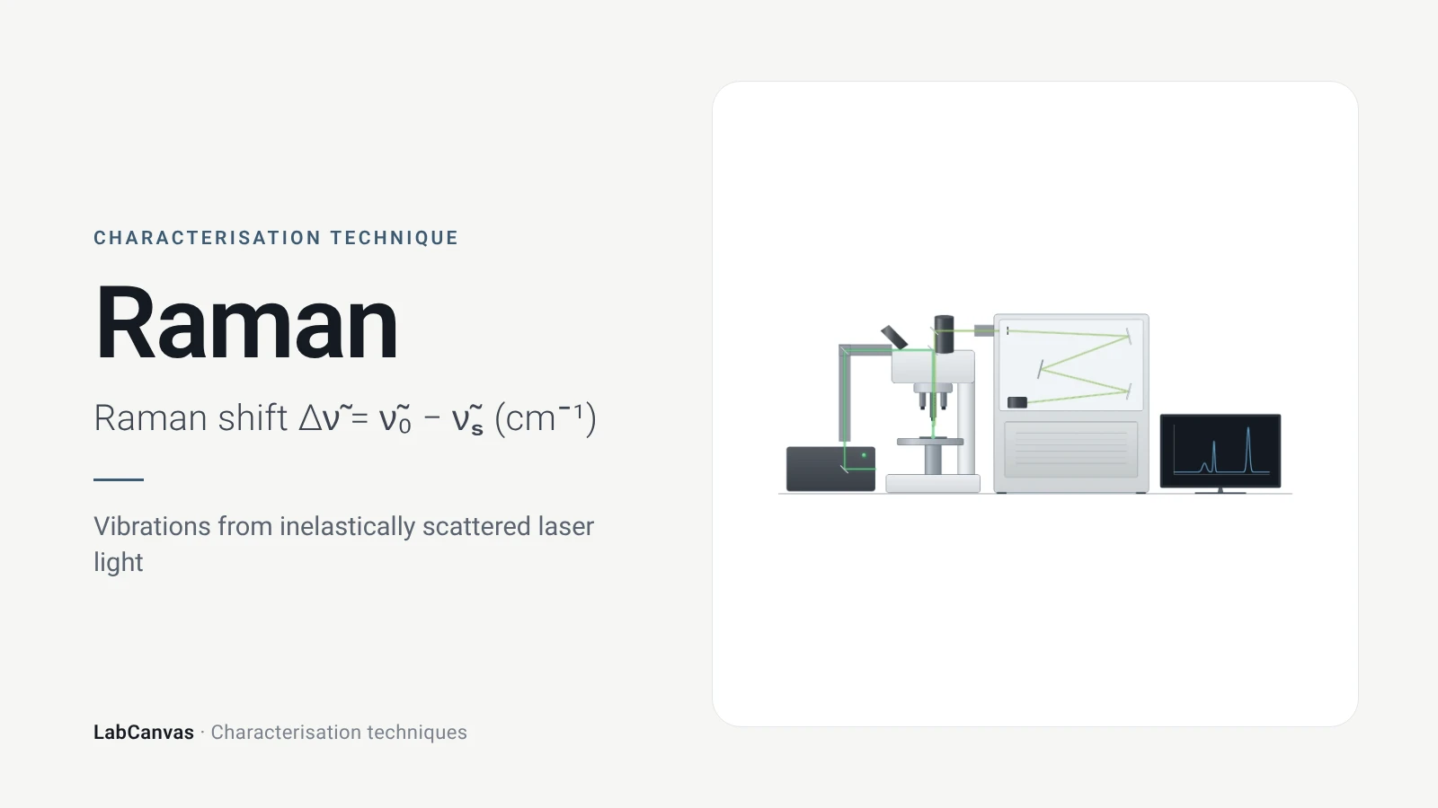
Raman: Vibrations from inelastically scattered laser light (Raman shift Δν̃ = ν̃₀ − ν̃ₛ (cm⁻¹))

TechniqueRaman shift Δν̃ = ν̃₀ − ν̃ₛ (cm⁻¹)

Raman spectroscopy

Raman spectroscopy explained: inelastic laser scattering, Raman shift, Stokes lines, IR complementarity, graphene D, G and 2D bands, lasers, fluorescence.

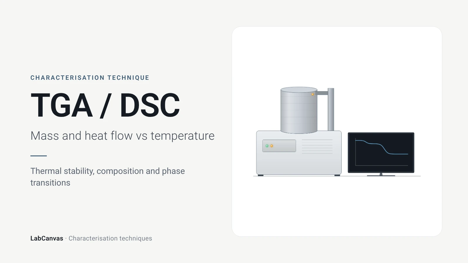
TGA / DSC: Thermal stability, composition and phase transitions (Mass and heat flow vs temperature)

TechniqueMass and heat flow vs temperature

TGA and DSC (thermal analysis)

TGA and DSC explained: mass loss and DTG vs temperature, atmosphere, MOF thermal stability, and glass transition, melting and crystallisation in DSC.

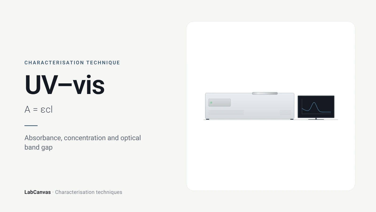
UV–vis: Absorbance, concentration and optical band gap (A = εcl)

TechniqueA = εcl

UV–vis spectroscopy

UV–vis spectroscopy explained: absorbance and the Beer–Lambert law, band gap from a Tauc plot, diffuse reflectance for powders and gold plasmon bands.

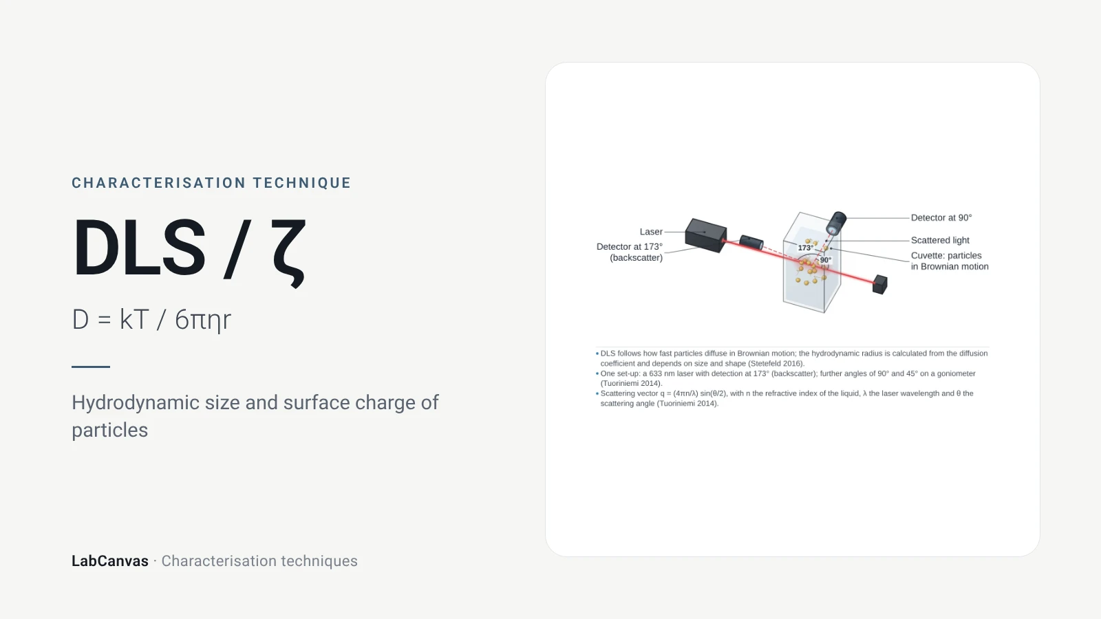
DLS / ζ: Hydrodynamic size and surface charge of particles (D = kT / 6πηr)

TechniqueD = kT / 6πηr

DLS and zeta potential

DLS and zeta potential explained: Brownian motion, Stokes–Einstein hydrodynamic size, intensity vs number distributions, PDI and colloidal stability.

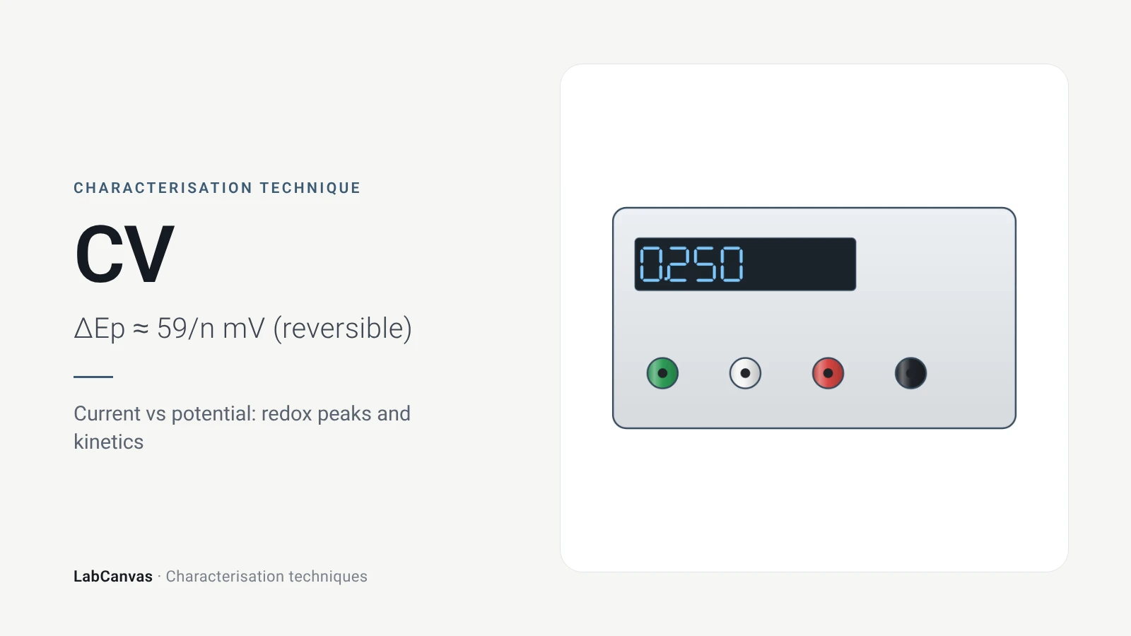
CV: Current vs potential: redox peaks and kinetics (ΔEp ≈ 59/n mV (reversible))

TechniqueΔEp ≈ 59/n mV (reversible)

Cyclic voltammetry (CV)

Cyclic voltammetry explained: three-electrode cell, scan rate, redox peaks, 59/n mV reversibility, Randles–Ševčík, RHE conversion, ECSA and Tafel pitfalls.

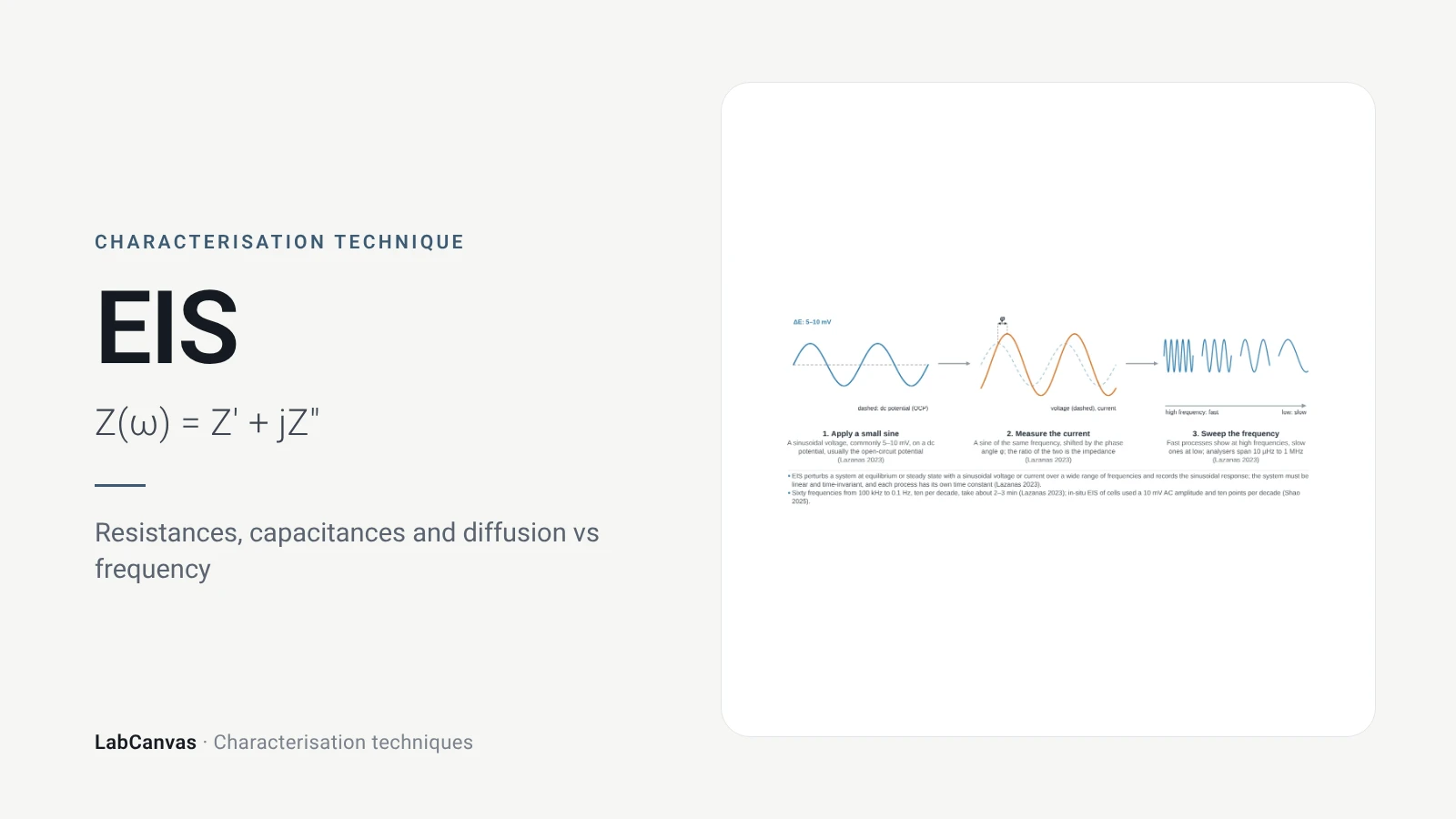
EIS: Resistances, capacitances and diffusion vs frequency (Z(ω) = Z′ + jZ″)

TechniqueZ(ω) = Z′ + jZ″

Electrochemical impedance spectroscopy (EIS)

EIS explained: small AC perturbation, Nyquist and Bode plots, Randles circuit, charge-transfer resistance, Warburg diffusion, batteries and catalysts.

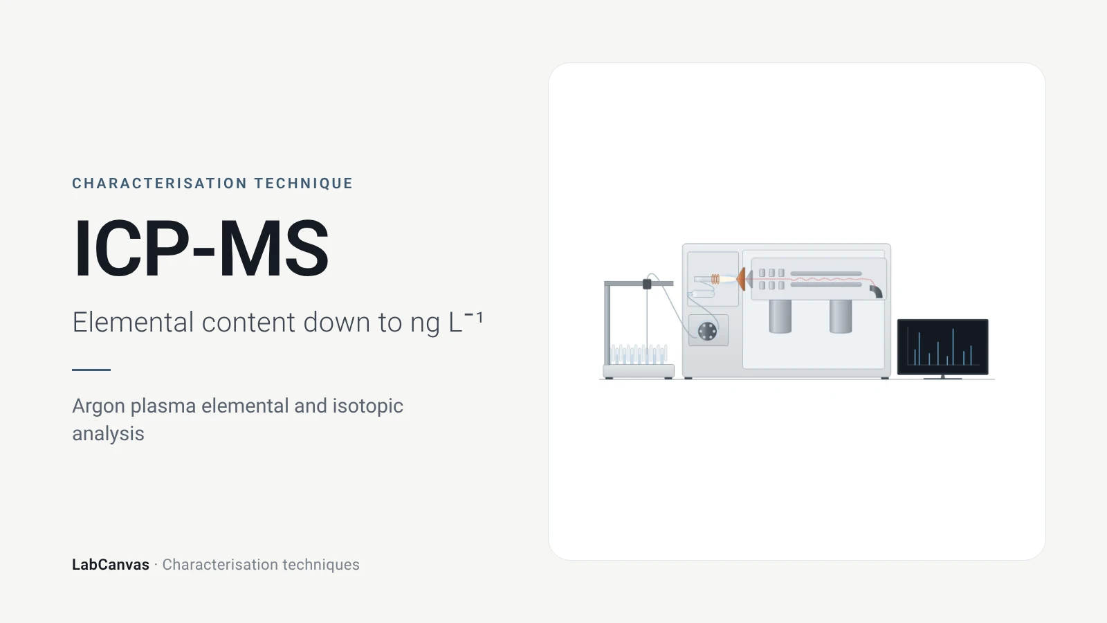
ICP-MS: Argon plasma elemental and isotopic analysis (Elemental content down to ng L⁻¹)

TechniqueElemental content down to ng L⁻¹

ICP-MS and ICP-OES

ICP-MS and ICP-OES explained: argon plasma, detection limits, acid digestion, interferences, single-particle ICP-MS and metal content of MOFs.

Frequently asked questions

What are the main materials characterisation techniques?

The core set is X-ray diffraction for crystal structure, electron microscopy (SEM and TEM) and AFM for morphology, XPS for surface chemistry, gas sorption (BET) for porosity, NMR, FTIR and Raman for bonding, TGA and DSC for thermal behaviour, UV–vis for optical properties, DLS for particle size in liquid, ICP-MS for composition, and cyclic voltammetry and EIS for electrochemistry. Each has its own page here with sources.

Which technique tells me if I made the right crystalline phase?

Powder X-ray diffraction: peak positions are set by the size and shape of the unit cell, so the measured pattern is compared with a simulated or published one to identify the phase and check purity (Abid et al. 2023).

What is the difference between SEM and TEM?

SEM scans a focused beam over the surface of a bulk sample and images topography and atomic-number contrast (Erlich et al. 2020); TEM sends electrons through a sample thinner than about 100 nm and resolves lattices, defects and diffraction (Bijelić et al. 2023).

What is the difference between XRD and XPS?

XRD measures long-range crystal structure averaged over the sample (Abid et al. 2023); XPS measures elements and their oxidation states in only the top 2–10 nm of the surface (Baio et al. 2020).

What is the difference between FTIR and Raman?

FTIR detects vibrations that change the dipole moment (Baker et al. 2014); Raman detects vibrations that change the polarisability, so the two are complementary; in centrosymmetric systems no mode is active in both (Jones et al. 2019).

Why do my DLS and TEM particle sizes not match?

DLS gives an intensity-weighted hydrodynamic diameter in liquid, which strongly favours large particles because scattering scales with d⁶ (Wishard & Gibb 2019); TEM measures dry cores. Differences of 200–300% are common (Filippov et al. 2023).

Which characterisation techniques are used for MOFs?

PXRD for phase, TGA for stability and the activation temperature, N₂ sorption at 77 K for the BET area, FTIR to check activation (Abid et al. 2023), digestion NMR for linker defects (Nerli et al. 2025) and low-dose TEM for atomic detail (Zheng et al. 2023).

How do I make a figure of characterisation data?

Each technique page has an editable instrument drawing and an example plot in LabCanvas; open them in the figure editor, replace the data with your own and export at journal resolution.

References

Z. Wang, G. Li, J. Zhang, Y. Wang, R. Sun, J. Lin. Energy-dispersive X-ray diffraction: principles, instrumentation and emerging applications. Materials 2026, 19, 697. doi:10.3390/ma19040697
H. R. Abid, M. R. Azhar, S. Iglauer, Z. H. Rada, A. Al-Yaseri, A. Keshavarz. Physiochemical characterization of metal organic framework materials: a mini review. Heliyon 2023, 10, e23840. doi:10.1016/j.heliyon.2023.e23840
J. E. Baio, D. J. Graham, D. G. Castner. Surface analysis tools for characterizing biological materials. Chem. Soc. Rev. 2020, 49, 3278–3296. doi:10.1039/d0cs00181c
J. W. M. Osterrieth et al.. How reproducible are surface areas calculated from the BET equation?. Adv. Mater. 2022, 34, e2201502. doi:10.1002/adma.202201502
M. Erlich, T. Arie, N. Koifman, Y. Talmon. Structure elucidation of silica-based core-shell microencapsulated drugs for topical applications by cryogenic scanning electron microscopy. J. Colloid Interface Sci. 2020, 579, 778–785. doi:10.1016/j.jcis.2020.06.114
L. Bijelić, F. Ruiz-Zepeda, N. Hodnik. The role of high-resolution transmission electron microscopy and aberration corrected scanning transmission electron microscopy in unraveling the structure–property relationships of Pt-based fuel cells electrocatalysts. Inorg. Chem. Front. 2023, 11, 323–341. doi:10.1039/d3qi01998e
S. Joo et al.. Atomic force microscopy for cross-disciplinary materials research. Small Methods 2025, 9, e2500514. doi:10.1002/smtd.202500514
D. E. Newbury, N. W. M. Ritchie. Performing elemental microanalysis with high accuracy and high precision by scanning electron microscopy/silicon drift detector energy-dispersive X-ray spectrometry (SEM/SDD-EDS). J. Mater. Sci. 2015, 50, 493–518. doi:10.1007/s10853-014-8685-2
E. Brunner, M. Rauche. Solid-state NMR spectroscopy: an advancing tool to analyse the structure and properties of metal–organic frameworks. Chem. Sci. 2020, 11, 4297–4304. doi:10.1039/d0sc00735h
G. F. Pauli et al.. Importance of purity evaluation and the potential of quantitative ¹H NMR as a purity assay. J. Med. Chem. 2014, 57, 9220–9231. doi:10.1021/jm500734a
M. J. Baker et al.. Using Fourier transform IR spectroscopy to analyze biological materials. Nat. Protoc. 2014, 9, 1771–1791. doi:10.1038/nprot.2014.110
R. R. Jones, D. C. Hooper, L. Zhang, D. Wolverson, V. K. Valev. Raman techniques: fundamentals and frontiers. Nanoscale Res. Lett. 2019, 14, 231. doi:10.1186/s11671-019-3039-2
C. Leyva-Porras et al.. Application of differential scanning calorimetry (DSC) and modulated differential scanning calorimetry (MDSC) in food and drug industries. Polymers 2019, 12, 5. doi:10.3390/polym12010005
T. G. Mayerhöfer, A. V. Pipa, J. Popp. Beer's law—why integrated absorbance depends linearly on concentration. ChemPhysChem 2019, 20, 2748–2753. doi:10.1002/cphc.201900787
A. Escobedo-Morales, I. I. Ruiz-López, M. de L. Ruiz-Peralta, L. Tepech-Carrillo, M. Sánchez-Cantú, J. E. Moreno-Orea. Automated method for the determination of the band gap energy of pure and mixed powder samples using diffuse reflectance spectroscopy. Heliyon 2019, 5, e01505. doi:10.1016/j.heliyon.2019.e01505
A. Wishard, B. C. Gibb. Dynamic light scattering – an all-purpose guide for the supramolecular chemist. Supramol. Chem. 2019, 31, 608–615. doi:10.1080/10610278.2019.1629438
J. Rodriguez-Loya, M. Lerma, J. L. Gardea-Torresdey. Dynamic light scattering and its application to control nanoparticle aggregation in colloidal systems: a review. Micromachines 2023, 15, 24. doi:10.3390/mi15010024
M. Rafiee, D. J. Abrams, L. Cardinale, Z. Goss, A. Romero-Arenas, S. S. Stahl. Cyclic voltammetry and chronoamperometry: mechanistic tools for organic electrosynthesis. Chem. Soc. Rev. 2024, 53, 566–585. doi:10.1039/d2cs00706a
A. Ch. Lazanas, M. I. Prodromidis. Electrochemical impedance spectroscopy—a tutorial. ACS Meas. Sci. Au 2023, 3, 162–193. doi:10.1021/acsmeasuresciau.2c00070
E. C. Mazarakioti, A. Zotos, A.-A. Thomatou, A. Kontogeorgos, A. Patakas, A. Ladavos. Inductively coupled plasma-mass spectrometry (ICP-MS), a useful tool in authenticity of agricultural products’ and foods’ origin. Foods 2022, 11, 3705. doi:10.3390/foods11223705
A. C. Ferrari et al.. Raman spectrum of graphene and graphene layers. Phys. Rev. Lett. 2006, 97, 187401. doi:10.1103/PhysRevLett.97.187401
I. M. Armitage, T. Drakenberg, B. Reilly. Use of ¹¹³Cd NMR to probe the native metal binding sites in metalloproteins: an overview. Met. Ions Life Sci. 2013, 11, 117–144. doi:10.1007/978-94-007-5179-8_6
D. A. Gómez-Gualdrón, P. Z. Moghadam, J. T. Hupp, O. K. Farha, R. Q. Snurr. Application of consistency criteria to calculate BET areas of micro- and mesoporous metal-organic frameworks. J. Am. Chem. Soc. 2016, 138, 215–224. doi:10.1021/jacs.5b10266
H. Y. Jeong, J. H. Lee, K. F. Hayes. Characterization of synthetic nanocrystalline mackinawite: crystal structure, particle size, and specific surface area. Geochim. Cosmochim. Acta 2008, 72, 493–505. doi:10.1016/j.gca.2007.11.008
S. K. Filippov et al.. Dynamic light scattering and transmission electron microscopy in drug delivery: a roadmap for correct characterization of nanoparticles and interpretation of results. Mater. Horiz. 2023, 10, 5354–5370. doi:10.1039/d3mh00717k
A. Zheng, K. Yin, R. Pan, M. Zhu, Y. Xiong, L. Sun. Research progress on metal-organic frameworks by advanced transmission electron microscopy. Nanomaterials 2023, 13, 1742. doi:10.3390/nano13111742
F. Nerli, V. Guiotto, V. Crocellà, M. Lessi, M. Taddei. Systematic assessment of the structural impact of linker fluorination in Ce-based UiO-66. Inorg. Chem. 2025, 64, 19688–19696. doi:10.1021/acs.inorgchem.5c03047

Draw Characterisation techniques figures for your paper

LabCanvas is a browser workspace for scientific figures: instruments with their beam and light paths, editable data plots, crystal structures, graphs and graphical abstracts at journal sizes.

Draw Characterisation techniques in LabCanvas