TikZ coordinates, paths, \foreach, scopes and styles
Quick answer
(2,1) is 2 cm right and 1 cm up, (30:2) is 2 cm at 30° (polar), ++(1,0) is 1 cm right of the previous point and moves there, and +(1,0) does the same without moving. Name a point with \coordinate (A) at (2,1); and compute new ones with the calc library, such as the midpoint ($(A)!0.5!(B)$). A path joins points with --, .. controls .. or to; \foreach repeats code, a scope groups options and transformations, and \tikzset{name/.style={…}} defines a reusable style.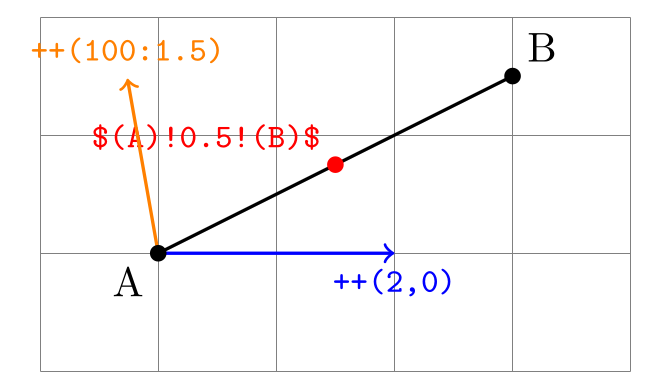
\usepackage{tikz} \usetikzlibrary{calc}\begin{tikzpicture}
\draw[help lines] (0,0) grid (5,3);
\coordinate (A) at (1,1); % a named point
\coordinate (B) at (4,2.5);
\draw[thick] (A) -- (B);
\fill[red] ($(A)!0.5!(B)$) circle (2pt) % calc: halfway from A to B
node[above left, font=\footnotesize\ttfamily] {\$(A)!0.5!(B)\$};
\draw[->, thick, blue] (A) -- ++(2,0) % relative: 2 cm to the right
node[below, font=\footnotesize\ttfamily] {++(2,0)};
\draw[->, thick, orange] (A) -- ++(100:1.5) % polar: 1.5 cm at 100 degrees
node[above, font=\footnotesize\ttfamily] {++(100:1.5)};
\fill (A) circle (2pt) node[below left] {A};
\fill (B) circle (2pt) node[above right] {B};
\end{tikzpicture}Full document
\documentclass[border=4pt]{standalone}
\usepackage{tikz}
\usetikzlibrary{calc}
\begin{document}
\begin{tikzpicture}
  \draw[help lines] (0,0) grid (5,3);
  \coordinate (A) at (1,1);                     % a named point
  \coordinate (B) at (4,2.5);
  \draw[thick] (A) -- (B);
  \fill[red] ($(A)!0.5!(B)$) circle (2pt)       % calc: halfway from A to B
    node[above left, font=\footnotesize\ttfamily] {\$(A)!0.5!(B)\$};
  \draw[->, thick, blue] (A) -- ++(2,0)         % relative: 2 cm to the right
    node[below, font=\footnotesize\ttfamily] {++(2,0)};
  \draw[->, thick, orange] (A) -- ++(100:1.5)   % polar: 1.5 cm at 100 degrees
    node[above, font=\footnotesize\ttfamily] {++(100:1.5)};
  \fill (A) circle (2pt) node[below left] {A};
  \fill (B) circle (2pt) node[above right] {B};
\end{tikzpicture}
\end{document}Contents
Cartesian and polar coordinates
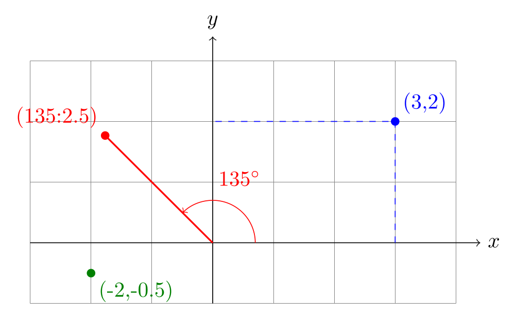
TikZ measures from the origin (0,0), with x to the right and y up. (3,2) is a point in the xy coordinate system: 3 times the x vector plus 2 times the y vector, and both vectors are initially 1 cm long, so plain numbers are centimetres. Negative values go left and down. A third number, (1,2,3), uses the xyz system, where the z vector initially points down-left (−3.85mm, −3.85mm), for simple 3D drawings.
A polar coordinate is (angle:radius): (135:2.5) is 2.5 cm from the origin in the direction 135°, with angles counted counter-clockwise from the positive x axis. (30:1cm and 2cm) gives different x and y radii, a point on an ellipse.
\usepackage{tikz}\begin{tikzpicture}
\draw[help lines] (-3,-1) grid (4,3);
\draw[->] (-3,0) -- (4.4,0) node[right] {$x$};
\draw[->] (0,-1) -- (0,3.4) node[above] {$y$};
% Cartesian (x,y): 3 cm right, 2 cm up
\draw[dashed, blue] (3,0) |- (0,2);
\fill[blue] (3,2) circle (2pt) node[above right] {(3,2)};
% polar (angle:radius): 2.5 cm at 135 degrees
\draw[red, thick] (0,0) -- (135:2.5);
\draw[red, ->] (0.7,0) arc[start angle=0, end angle=135, radius=0.7];
\node[red] at (67.5:1.15) {$135^\circ$};
\fill[red] (135:2.5) circle (2pt) node[above left] {(135:2.5)};
% negative values go left and down
\fill[green!50!black] (-2,-0.5) circle (2pt) node[below right] {(-2,-0.5)};
\end{tikzpicture}Full document
\documentclass[border=4pt]{standalone}
\usepackage{tikz}
\begin{document}
\begin{tikzpicture}
  \draw[help lines] (-3,-1) grid (4,3);
  \draw[->] (-3,0) -- (4.4,0) node[right] {$x$};
  \draw[->] (0,-1) -- (0,3.4) node[above] {$y$};
  % Cartesian (x,y): 3 cm right, 2 cm up
  \draw[dashed, blue] (3,0) |- (0,2);
  \fill[blue] (3,2) circle (2pt) node[above right] {(3,2)};
  % polar (angle:radius): 2.5 cm at 135 degrees
  \draw[red, thick] (0,0) -- (135:2.5);
  \draw[red, ->] (0.7,0) arc[start angle=0, end angle=135, radius=0.7];
  \node[red] at (67.5:1.15) {$135^\circ$};
  \fill[red] (135:2.5) circle (2pt) node[above left] {(135:2.5)};
  % negative values go left and down
  \fill[green!50!black] (-2,-0.5) circle (2pt) node[below right] {(-2,-0.5)};
\end{tikzpicture}
\end{document}Units, the x and y vectors, and scale
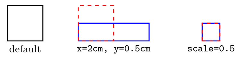
A number with a unit, (1cm,2pt), is a point in the canvas system and is taken literally. A number without a unit is multiplied by the x or y vector, which the options x=… and y=… change: in [x=2cm, y=0.5cm], (1,1) becomes 2 cm by 0.5 cm, while (1cm,1cm) stays a 1 cm square, as the middle picture shows. scale=0.5 is different: it is a transformation, so it shrinks every coordinate, with or without units (right). Line widths and node text are not scaled by either.
\usepackage{tikz}\begin{tikzpicture}[font=\footnotesize]
% default: 1 unit = 1 cm in both directions
\draw[thick] (0,0) rectangle (1,1);
\node[below] at (0.5,0) {default};
% new unit vectors stretch plain numbers, not lengths with units
\begin{scope}[xshift=2cm, x=2cm, y=0.5cm]
\draw[thick, blue] (0,0) rectangle (1,1); % 2 cm by 0.5 cm
\draw[thick, red, dashed] (0,0) rectangle (1cm,1cm); % still 1 cm square
\end{scope}
\node[below, align=center] at (3,0) {\texttt{x=2cm, y=0.5cm}};
% scale transforms every coordinate, with or without units
\begin{scope}[xshift=5.5cm, scale=0.5]
\draw[thick, blue] (0,0) rectangle (1,1);
\draw[thick, red, dashed] (0,0) rectangle (1cm,1cm);
\end{scope}
\node[below] at (5.75,0) {\texttt{scale=0.5}};
\end{tikzpicture}Full document
\documentclass[border=4pt]{standalone}
\usepackage{tikz}
\begin{document}
\begin{tikzpicture}[font=\footnotesize]
  % default: 1 unit = 1 cm in both directions
  \draw[thick] (0,0) rectangle (1,1);
  \node[below] at (0.5,0) {default};
  % new unit vectors stretch plain numbers, not lengths with units
  \begin{scope}[xshift=2cm, x=2cm, y=0.5cm]
    \draw[thick, blue] (0,0) rectangle (1,1);              % 2 cm by 0.5 cm
    \draw[thick, red, dashed] (0,0) rectangle (1cm,1cm);   % still 1 cm square
  \end{scope}
  \node[below, align=center] at (3,0) {\texttt{x=2cm, y=0.5cm}};
  % scale transforms every coordinate, with or without units
  \begin{scope}[xshift=5.5cm, scale=0.5]
    \draw[thick, blue] (0,0) rectangle (1,1);
    \draw[thick, red, dashed] (0,0) rectangle (1cm,1cm);
  \end{scope}
  \node[below] at (5.75,0) {\texttt{scale=0.5}};
\end{tikzpicture}
\end{document}Relative coordinates: + and ++
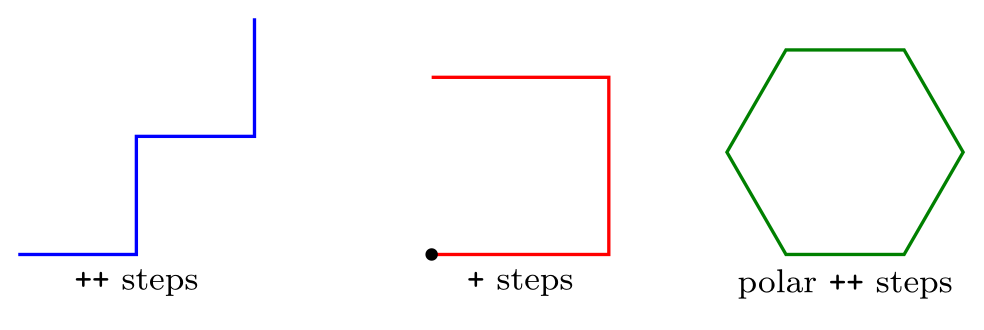
++(dx,dy) is measured from the previous point and then becomes the current point, so a chain of ++ steps walks along: (0,0) -- ++(1,0) -- ++(0,1) is a staircase. +(dx,dy) is also measured from the previous point but does not move it, so every + step in a row starts from the same place: the red path below goes to three corners of a square, all measured from its start. Relative steps work with polar coordinates too, which makes regular shapes easy: six steps of ++(\a:1) with the angle growing by 60° draw a hexagon.
Two special cases from the manual: inside .. controls .. a relative control point is measured from the start of the curve (first control point) or from its end (second control point), and ([turn]30:1cm) turns the axes so that 0° points along the direction the path arrived from.
\usepackage{tikz}\begin{tikzpicture}[font=\footnotesize]
% ++ moves on: each step starts where the last one ended
\draw[thick, blue] (0,0) -- ++(1,0) -- ++(0,1) -- ++(1,0) -- ++(0,1);
\node[below] at (1,0) {\texttt{++} steps};
% + does not move: every step is measured from (3.5,0)
\draw[thick, red] (3.5,0) -- +(1.5,0) -- +(1.5,1.5) -- +(0,1.5);
\fill (3.5,0) circle (1.5pt);
\node[below] at (4.25,0) {\texttt{+} steps};
% relative polar steps inside a loop: a regular hexagon
\draw[thick, green!50!black] (6.5,0)
\foreach \a in {0,60,...,240} { -- ++(\a:1) } -- cycle;
\node[below] at (7,0) {polar \texttt{++} steps};
\end{tikzpicture}Full document
\documentclass[border=4pt]{standalone}
\usepackage{tikz}
\begin{document}
\begin{tikzpicture}[font=\footnotesize]
  % ++ moves on: each step starts where the last one ended
  \draw[thick, blue] (0,0) -- ++(1,0) -- ++(0,1) -- ++(1,0) -- ++(0,1);
  \node[below] at (1,0) {\texttt{++} steps};
  % + does not move: every step is measured from (3.5,0)
  \draw[thick, red] (3.5,0) -- +(1.5,0) -- +(1.5,1.5) -- +(0,1.5);
  \fill (3.5,0) circle (1.5pt);
  \node[below] at (4.25,0) {\texttt{+} steps};
  % relative polar steps inside a loop: a regular hexagon
  \draw[thick, green!50!black] (6.5,0)
    \foreach \a in {0,60,...,240} { -- ++(\a:1) } -- cycle;
  \node[below] at (7,0) {polar \texttt{++} steps};
\end{tikzpicture}
\end{document}Named coordinates and node anchors
\coordinate (A) at (2,1); names a point; inside a path, (2,1) coordinate (A) does the same. Afterwards (A) can be used anywhere a coordinate is expected, which keeps a drawing easy to change. Every named node is also a coordinate: (box) alone means its centre, but a line drawn to it stops at its border. Anchors pick other points: (box.north), (box.south west), (box.east), or an angle, (box.30), the border point in the direction 30° from the centre.
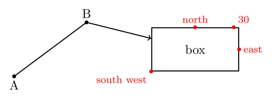
\usepackage{tikz}\begin{tikzpicture}
\coordinate (A) at (0,0);
\coordinate (B) at (2,1.5);
\node[draw, thick, minimum width=2.4cm, minimum height=1.2cm] (box) at (5,0.75) {box};
\draw[thick] (A) -- (B); % named coordinates
\draw[thick, ->] (B) -- (box); % a node name: the line stops at the border
% anchors of a node: (box.north), (box.south west), (box.30) ...
\foreach \a/\where in {north/above, south west/below left, east/right, 30/above right}
\fill[red] (box.\a) circle (1.5pt) node[\where, font=\footnotesize] {\a};
\fill (A) circle (1.5pt) node[below] {A};
\fill (B) circle (1.5pt) node[above] {B};
\end{tikzpicture}Full document
\documentclass[border=4pt]{standalone}
\usepackage{tikz}
\begin{document}
\begin{tikzpicture}
  \coordinate (A) at (0,0);
  \coordinate (B) at (2,1.5);
  \node[draw, thick, minimum width=2.4cm, minimum height=1.2cm] (box) at (5,0.75) {box};
  \draw[thick] (A) -- (B);           % named coordinates
  \draw[thick, ->] (B) -- (box);     % a node name: the line stops at the border
  % anchors of a node: (box.north), (box.south west), (box.30) ...
  \foreach \a/\where in {north/above, south west/below left, east/right, 30/above right}
    \fill[red] (box.\a) circle (1.5pt) node[\where, font=\footnotesize] {\a};
  \fill (A) circle (1.5pt) node[below] {A};
  \fill (B) circle (1.5pt) node[above] {B};
\end{tikzpicture}
\end{document}Computing coordinates with the calc library
With \usetikzlibrary{calc}, a coordinate between ($ and $) is computed. The most used forms:
| Expression | Result |
|---|---|
($(A)!0.5!(B)$) | the point halfway from A to B (0 is A, 1 is B; 0.25 a quarter of the way, 1.5 beyond B) |
($(A)!1cm!(B)$) | 1 cm from A towards B |
($(A)!(C)!(B)$) | C projected onto the line AB (the foot of the perpendicular) |
($(A) + (1,2)$), ($(A) - (B)$) | sums and differences of points |
($2*(A)$), ($1/3*(A) + 1/3*(B) + 1/3*(C)$) | a factor before a coordinate scales it; here the centroid of a triangle |
($(A)!0.5!30:(B)$) | B is first rotated by 30° around A, then the partway modifier applies |
A factor that starts with a parenthesis must be put in braces, as in {(1+2)/2}*(A), because a computation that starts with ( is read as a coordinate. Without the library, a ($…$) coordinate stops with an error that names the missing line. For computations in the middle of a path, the let operation stores points and numbers, for example let \p1 = ($(B)-(A)$) in, after which \x1 and \y1 are its components.
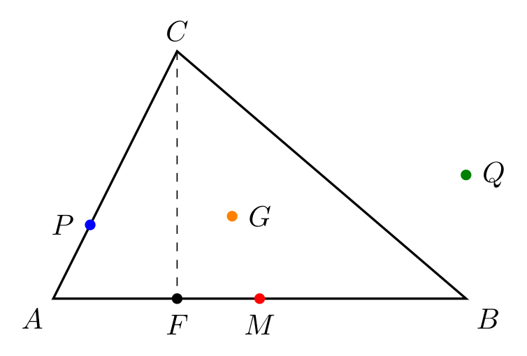
\usepackage{tikz} \usetikzlibrary{calc}\begin{tikzpicture}[dot/.style={circle, fill, inner sep=1.3pt}]
\coordinate (A) at (0,0);
\coordinate (B) at (5,0);
\coordinate (C) at (1.5,3);
\draw[thick] (A) -- (B) -- (C) -- cycle;
\node[dot, red, label=below:$M$] at ($(A)!0.5!(B)$) {}; % halfway from A to B
\node[dot, blue, label=left:$P$] at ($(A)!1cm!(C)$) {}; % 1 cm from A towards C
\draw[dashed] (C) -- ($(A)!(C)!(B)$) node[dot, label=below:$F$] {}; % C projected onto AB
\node[dot, orange, label=right:$G$] at ($1/3*(A) + 1/3*(B) + 1/3*(C)$) {}; % centroid
\node[dot, green!50!black, label=right:$Q$] at ($(B) + (0,1.5)$) {}; % B moved up
\path (A) node[below left] {$A$} (B) node[below right] {$B$} (C) node[above] {$C$};
\end{tikzpicture}Full document
\documentclass[border=4pt]{standalone}
\usepackage{tikz}
\usetikzlibrary{calc}
\begin{document}
\begin{tikzpicture}[dot/.style={circle, fill, inner sep=1.3pt}]
  \coordinate (A) at (0,0);
  \coordinate (B) at (5,0);
  \coordinate (C) at (1.5,3);
  \draw[thick] (A) -- (B) -- (C) -- cycle;
  \node[dot, red, label=below:$M$] at ($(A)!0.5!(B)$) {};       % halfway from A to B
  \node[dot, blue, label=left:$P$] at ($(A)!1cm!(C)$) {};       % 1 cm from A towards C
  \draw[dashed] (C) -- ($(A)!(C)!(B)$) node[dot, label=below:$F$] {}; % C projected onto AB
  \node[dot, orange, label=right:$G$] at ($1/3*(A) + 1/3*(B) + 1/3*(C)$) {}; % centroid
  \node[dot, green!50!black, label=right:$Q$] at ($(B) + (0,1.5)$) {};     % B moved up
  \path (A) node[below left] {$A$} (B) node[below right] {$B$} (C) node[above] {$C$};
\end{tikzpicture}
\end{document}Intersections of lines and paths
For the frequent case of a vertical and a horizontal line there is a built-in syntax: (P |- Q) is the point with the x of P and the y of Q, and (P -| Q) the other way round; the manual’s example is (2,1 |- 3,4), which is (2,4). This needs no library and is the usual way to align nodes or draw right-angled connectors.
For any two paths, load \usetikzlibrary{intersections}, give each path a name path=…, and then name intersections={of=a and b} on a later path defines the coordinates (intersection-1), (intersection-2), … total=\t stores how many there are, by={X,Y} gives them your own names. The manual warns that because of TeX’s limited accuracy the paths should not be too complicated: plots and decorated paths made of many tiny segments are poor candidates.
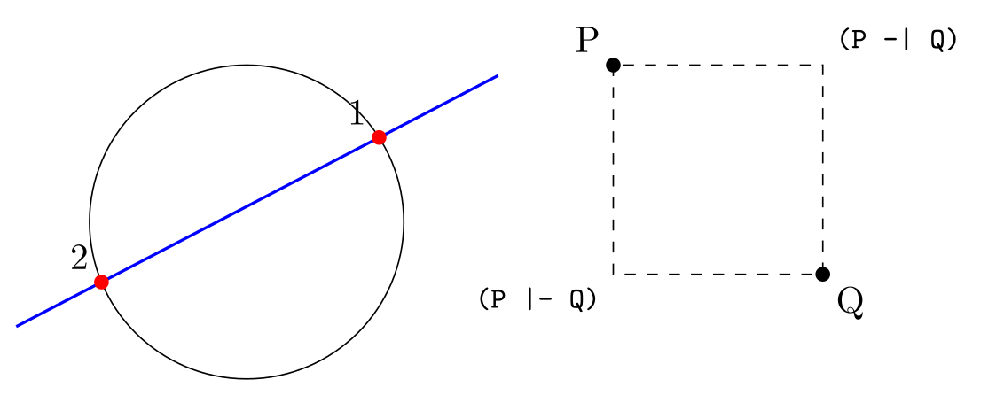
\usepackage{tikz} \usetikzlibrary{intersections}\begin{tikzpicture}
% any two named paths: the intersections library
\draw[name path=circle] (0,0) circle[radius=1.5];
\draw[name path=line, thick, blue] (-2.2,-1) -- (2.4,1.4);
\fill[red, name intersections={of=circle and line, total=\t}]
\foreach \i in {1,...,\t} {(intersection-\i) circle (2pt) node[above left, text=black] {\i}};
% perpendicular lines: no library needed
\coordinate (P) at (3.5,1.5);
\coordinate (Q) at (5.5,-0.5);
\draw[dashed] (P) -- (P |- Q) -- (Q) -- (P -| Q) -- cycle;
\fill (P) circle (2pt) node[above left] {P};
\fill (Q) circle (2pt) node[below right] {Q};
\node[below left, font=\footnotesize] at (P |- Q) {\texttt{(P |- Q)}};
\node[above right, font=\footnotesize] at (P -| Q) {\texttt{(P -| Q)}};
\end{tikzpicture}Full document
\documentclass[border=4pt]{standalone}
\usepackage{tikz}
\usetikzlibrary{intersections}
\begin{document}
\begin{tikzpicture}
  % any two named paths: the intersections library
  \draw[name path=circle] (0,0) circle[radius=1.5];
  \draw[name path=line, thick, blue] (-2.2,-1) -- (2.4,1.4);
  \fill[red, name intersections={of=circle and line, total=\t}]
    \foreach \i in {1,...,\t} {(intersection-\i) circle (2pt) node[above left, text=black] {\i}};
  % perpendicular lines: no library needed
  \coordinate (P) at (3.5,1.5);
  \coordinate (Q) at (5.5,-0.5);
  \draw[dashed] (P) -- (P |- Q) -- (Q) -- (P -| Q) -- cycle;
  \fill (P) circle (2pt) node[above left] {P};
  \fill (Q) circle (2pt) node[below right] {Q};
  \node[below left, font=\footnotesize] at (P |- Q) {\texttt{(P |- Q)}};
  \node[above right, font=\footnotesize] at (P -| Q) {\texttt{(P -| Q)}};
\end{tikzpicture}
\end{document}Paths and path operations
A path is a sequence of coordinates and operations ending with a semicolon. The command decides what happens to it: \draw strokes it, \fill fills it, \filldraw does both, \shade shades it, \clip clips everything after it in the scope, and \path does nothing visible (it is \path[draw] that \draw abbreviates), which is useful for placing nodes or naming paths.
| Operation | What it adds |
|---|---|
(a) -- (b) | a straight line |
(a) -| (b), (a) |- (b) | horizontal then vertical, or vertical then horizontal |
-- cycle | closes the path back to its start with proper corners (needed for clean fills and joins) |
(a) rectangle (b) | a rectangle with opposite corners a and b |
circle[radius=1], ellipse[x radius=2, y radius=1] | around the current point |
arc[start angle=0, end angle=90, radius=1] | an arc starting at the current point |
.. controls (c) and (d) .. (b) | a cubic Bézier curve |
to[out=…, in=…], to[bend left] | a curve set by its angles, or a straight line without options |
grid, parabola, sin, cos, plot | grids, parabolas, sine curves and function plots |
node, coordinate, pic, edge | text, names, small pictures and extra lines placed along the path |
A coordinate without an operation before it is a move-to: \draw (0,0) -- (1,0) (2,0) -- (3,0); draws two separate pieces with one command, which then share their options.
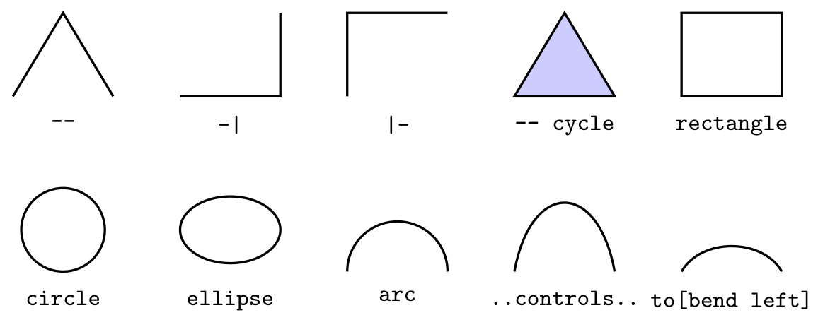
\usepackage{tikz}\begin{tikzpicture}[thick, every node/.style={font=\footnotesize\ttfamily, below}]
\draw (0,0) -- (0.6,1) -- (1.2,0); \node at (0.6,-0.1) {--};
\draw (2,0) -| (3.2,1); \node at (2.6,-0.1) {-|};
\draw (4,0) |- (5.2,1); \node at (4.6,-0.1) {|-};
\filldraw[fill=blue!20] (6,0) -- (7.2,0) -- (6.6,1) -- cycle;
\node at (6.6,-0.1) {-- cycle};
\draw (8,0) rectangle (9.2,1); \node at (8.6,-0.1) {rectangle};
\draw (0.6,-1.6) circle[radius=0.5]; \node at (0.6,-2.2) {circle};
\draw (2.6,-1.6) ellipse[x radius=0.6, y radius=0.4]; \node at (2.6,-2.2) {ellipse};
\draw (5.2,-2.1) arc[start angle=0, end angle=180, radius=0.6];
\node at (4.6,-2.2) {arc};
\draw (6,-2.1) .. controls (6.2,-1) and (7,-1) .. (7.2,-2.1);
\node at (6.6,-2.2) {..controls..};
\draw (8,-2.1) to[bend left=60] (9.2,-2.1); \node at (8.6,-2.2) {to[bend left]};
\end{tikzpicture}Full document
\documentclass[border=4pt]{standalone}
\usepackage{tikz}
\begin{document}
\begin{tikzpicture}[thick, every node/.style={font=\footnotesize\ttfamily, below}]
  \draw (0,0) -- (0.6,1) -- (1.2,0);              \node at (0.6,-0.1) {--};
  \draw (2,0) -| (3.2,1);                         \node at (2.6,-0.1) {-|};
  \draw (4,0) |- (5.2,1);                         \node at (4.6,-0.1) {|-};
  \filldraw[fill=blue!20] (6,0) -- (7.2,0) -- (6.6,1) -- cycle;
                                                  \node at (6.6,-0.1) {-- cycle};
  \draw (8,0) rectangle (9.2,1);                  \node at (8.6,-0.1) {rectangle};
  \draw (0.6,-1.6) circle[radius=0.5];            \node at (0.6,-2.2) {circle};
  \draw (2.6,-1.6) ellipse[x radius=0.6, y radius=0.4]; \node at (2.6,-2.2) {ellipse};
  \draw (5.2,-2.1) arc[start angle=0, end angle=180, radius=0.6];
                                                  \node at (4.6,-2.2) {arc};
  \draw (6,-2.1) .. controls (6.2,-1) and (7,-1) .. (7.2,-2.1);
                                                  \node at (6.6,-2.2) {..controls..};
  \draw (8,-2.1) to[bend left=60] (9.2,-2.1);     \node at (8.6,-2.2) {to[bend left]};
\end{tikzpicture}
\end{document}Bézier curves: .. controls ..
(a) .. controls (c) and (d) .. (b) draws a cubic Bézier curve from a to b. The curve leaves a heading towards the first control point c and arrives at b coming from the second control point d; the further away the control points are, the more the curve bulges. It does not pass through them. With only one control point, .. controls (c) .., the same point is used for both. With relative control points, .. controls +(60:1.5) and +(120:1.5) .., the first is measured from the start and the second from the end, so you can write the angles at which the curve leaves and arrives. cycle can end a curve, as in .. controls (1,1) .. cycle.
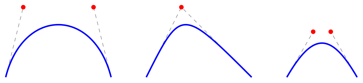
\usepackage{tikz}\begin{tikzpicture}[ctrl/.style={gray, dashed}, pt/.style={circle, fill=red, inner sep=1.3pt}]
% two control points: leaves towards the first, arrives from the second
\draw[ctrl] (0,0) -- (0.5,2) (2.5,2) -- (3,0);
\draw[very thick, blue] (0,0) .. controls (0.5,2) and (2.5,2) .. (3,0);
\node[pt] at (0.5,2) {}; \node[pt] at (2.5,2) {};
% one control point is used twice
\draw[ctrl] (4,0) -- (5,2) -- (7,0);
\draw[very thick, blue] (4,0) .. controls (5,2) .. (7,0);
\node[pt] at (5,2) {};
% relative control points: +() from the start, and from the end
\draw[ctrl] (8,0) -- +(60:1.5) node[pt] {} (10,0) -- +(120:1.5) node[pt] {};
\draw[very thick, blue] (8,0) .. controls +(60:1.5) and +(120:1.5) .. (10,0);
\end{tikzpicture}Full document
\documentclass[border=4pt]{standalone}
\usepackage{tikz}
\begin{document}
\begin{tikzpicture}[ctrl/.style={gray, dashed}, pt/.style={circle, fill=red, inner sep=1.3pt}]
  % two control points: leaves towards the first, arrives from the second
  \draw[ctrl] (0,0) -- (0.5,2) (2.5,2) -- (3,0);
  \draw[very thick, blue] (0,0) .. controls (0.5,2) and (2.5,2) .. (3,0);
  \node[pt] at (0.5,2) {}; \node[pt] at (2.5,2) {};
  % one control point is used twice
  \draw[ctrl] (4,0) -- (5,2) -- (7,0);
  \draw[very thick, blue] (4,0) .. controls (5,2) .. (7,0);
  \node[pt] at (5,2) {};
  % relative control points: +() from the start, and from the end
  \draw[ctrl] (8,0) -- +(60:1.5) node[pt] {} (10,0) -- +(120:1.5) node[pt] {};
  \draw[very thick, blue] (8,0) .. controls +(60:1.5) and +(120:1.5) .. (10,0);
\end{tikzpicture}
\end{document}Curves with to: out, in, bend and looseness
(a) to (b) without options is a straight line. to[out=90, in=180] leaves a at 90° and arrives at b from the direction 180°; looseness (initially 1) makes the curve wider or tighter. to[bend left] and to[bend right] bow the line to one side, by 30° unless you give an angle such as bend right=45. These are often easier than control points because you only state directions. to also takes nodes, (a) to node[above] {x} (b), and works with cycle.
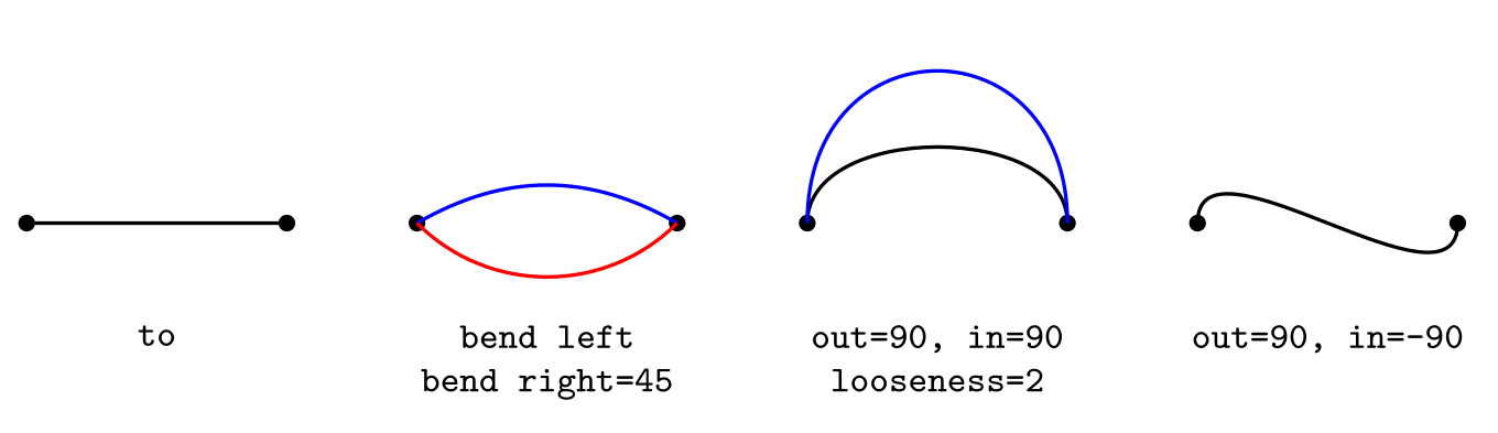
\usepackage{tikz}\begin{tikzpicture}[thick, pt/.style={circle, fill, inner sep=1.3pt},
lbl/.style={below=3pt, font=\footnotesize\ttfamily, align=center}]
\foreach \x in {0,3,6,9} { \node[pt] at (\x,0) {}; \node[pt] at (\x+2,0) {}; }
\draw (0,0) to (2,0);
\node[lbl] at (1,-0.55) {to};
\draw[blue] (3,0) to[bend left] (5,0);
\draw[red] (3,0) to[bend right=45] (5,0);
\node[lbl] at (4,-0.55) {bend left\\bend right=45};
\draw (6,0) to[out=90, in=90] (8,0);
\draw[blue] (6,0) to[out=90, in=90, looseness=2] (8,0);
\node[lbl] at (7,-0.55) {out=90, in=90\\looseness=2};
\draw (9,0) to[out=90, in=-90] (11,0);
\node[lbl] at (10,-0.55) {out=90, in=-90};
\end{tikzpicture}Full document
\documentclass[border=4pt]{standalone}
\usepackage{tikz}
\begin{document}
\begin{tikzpicture}[thick, pt/.style={circle, fill, inner sep=1.3pt},
                    lbl/.style={below=3pt, font=\footnotesize\ttfamily, align=center}]
  \foreach \x in {0,3,6,9} { \node[pt] at (\x,0) {}; \node[pt] at (\x+2,0) {}; }
  \draw (0,0) to (2,0);
  \node[lbl] at (1,-0.55) {to};
  \draw[blue] (3,0) to[bend left] (5,0);
  \draw[red] (3,0) to[bend right=45] (5,0);
  \node[lbl] at (4,-0.55) {bend left\\bend right=45};
  \draw (6,0) to[out=90, in=90] (8,0);
  \draw[blue] (6,0) to[out=90, in=90, looseness=2] (8,0);
  \node[lbl] at (7,-0.55) {out=90, in=90\\looseness=2};
  \draw (9,0) to[out=90, in=-90] (11,0);
  \node[lbl] at (10,-0.55) {out=90, in=-90};
\end{tikzpicture}
\end{document}\foreach: lists, ranges and steps
\foreach \x in {list} {commands} runs the commands once for each item, with \x set to it. Without braces, the commands run up to the next semicolon, so \foreach \x in {1,2,3} \draw (\x,0) circle (2pt); is a complete loop. The three dots fill in a range:
{1,...,6}is 1 to 6 in steps of 1 (and{6,...,1}counts down);{0,0.5,...,3}: the first two items set the step, here 0.5;{a,...,e}works for letters;- a macro can hold the list:
\def\mylist{1,3,7}and\foreach \x in \mylist.
Watch fractional steps: TeX arithmetic is not exact, and the manual’s own example {0,0.1,...,0.5} gives 0, 0.1, 0.20001, 0.30002, 0.40002, so the last value is missing. Make the end a little larger (0.501) or loop over integers and divide. Items that contain commas, such as pairs, are fine when they start with a parenthesis: \foreach \p in {(0,0), (1,1)}.
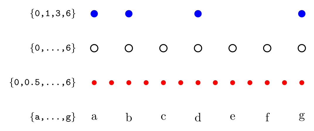
\usepackage{tikz}\begin{tikzpicture}[lbl/.style={left, font=\footnotesize\ttfamily}]
% a list of values
\foreach \x in {0,1,3,6} \fill[blue] (\x,3) circle (3pt);
\node[lbl] at (-0.4,3) {\{0,1,3,6\}};
% a range: 0, 1, 2, ..., 6
\foreach \x in {0,...,6} \draw[thick] (\x,2) circle (3pt);
\node[lbl] at (-0.4,2) {\{0,...,6\}};
% the first two items set the step: 0, 0.5, 1, ..., 6
\foreach \x in {0,0.5,...,6} \fill[red] (\x,1) circle (2pt);
\node[lbl] at (-0.4,1) {\{0,0.5,...,6\}};
% letters work too; count numbers the items
\foreach \l [count=\i] in {a,...,g} \node at (\i-1,0) {\l};
\node[lbl] at (-0.4,0) {\{a,...,g\}};
\end{tikzpicture}Full document
\documentclass[border=4pt]{standalone}
\usepackage{tikz}
\begin{document}
\begin{tikzpicture}[lbl/.style={left, font=\footnotesize\ttfamily}]
  % a list of values
  \foreach \x in {0,1,3,6} \fill[blue] (\x,3) circle (3pt);
  \node[lbl] at (-0.4,3) {\{0,1,3,6\}};
  % a range: 0, 1, 2, ..., 6
  \foreach \x in {0,...,6} \draw[thick] (\x,2) circle (3pt);
  \node[lbl] at (-0.4,2) {\{0,...,6\}};
  % the first two items set the step: 0, 0.5, 1, ..., 6
  \foreach \x in {0,0.5,...,6} \fill[red] (\x,1) circle (2pt);
  \node[lbl] at (-0.4,1) {\{0,0.5,...,6\}};
  % letters work too; count numbers the items
  \foreach \l [count=\i] in {a,...,g} \node at (\i-1,0) {\l};
  \node[lbl] at (-0.4,0) {\{a,...,g\}};
\end{tikzpicture}
\end{document}\foreach with several variables, count, evaluate and remember
\foreach \x/\c in {0/red, 1/blue} splits each item at the slash into several variables; an item with too few parts repeats its last part, so a plain 3 sets both to 3. Options go in square brackets after the variables:
[count=\i]numbers the items 1, 2, 3…;count=\i from 0starts elsewhere;[evaluate=\x as \y using 20*\x]computes a value (list items are not evaluated otherwise:1+2stays the text 1+2);[remember=\x as \last (initially A)]keeps the previous item, handy for joining consecutive nodes;[parse=true]lets the upper bound be an expression, as in{1,...,2*3}.
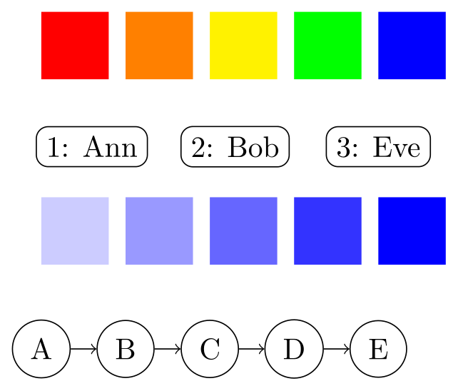
\usepackage{tikz}\begin{tikzpicture}
% two variables per item, separated by /
\foreach \x/\c in {0/red, 1/orange, 2/yellow, 3/green, 4/blue}
\fill[\c] (\x,0) rectangle +(0.8,0.8);
% count: the position of the item in the list
\foreach \name [count=\i] in {Ann, Bob, Eve}
\node[draw, rounded corners] at (1.7*\i - 1.1, -0.8) {\i: \name};
% evaluate: compute a value from the variable
\foreach \x [evaluate=\x as \pct using 20*\x] in {1,...,5}
\fill[blue!\pct] (\x - 1, -2.2) rectangle +(0.8,0.8);
% remember: the value from the previous round
\foreach \l [count=\i] in {A,...,E}
\node[circle, draw] (\l) at (\i - 1, -3.2) {\l};
\foreach \l [remember=\l as \prev (initially A)] in {B,...,E}
\draw[->] (\prev) -- (\l);
\end{tikzpicture}Full document
\documentclass[border=4pt]{standalone}
\usepackage{tikz}
\begin{document}
\begin{tikzpicture}
  % two variables per item, separated by /
  \foreach \x/\c in {0/red, 1/orange, 2/yellow, 3/green, 4/blue}
    \fill[\c] (\x,0) rectangle +(0.8,0.8);
  % count: the position of the item in the list
  \foreach \name [count=\i] in {Ann, Bob, Eve}
    \node[draw, rounded corners] at (1.7*\i - 1.1, -0.8) {\i: \name};
  % evaluate: compute a value from the variable
  \foreach \x [evaluate=\x as \pct using 20*\x] in {1,...,5}
    \fill[blue!\pct] (\x - 1, -2.2) rectangle +(0.8,0.8);
  % remember: the value from the previous round
  \foreach \l [count=\i] in {A,...,E}
    \node[circle, draw] (\l) at (\i - 1, -3.2) {\l};
  \foreach \l [remember=\l as \prev (initially A)] in {B,...,E}
    \draw[->] (\prev) -- (\l);
\end{tikzpicture}
\end{document}Nested loops and loops inside a path
A \foreach directly followed by another one is a nested loop: the inner loop runs completely for every value of the outer one. Each pass of the loop runs inside a TeX group, so definitions made in the body (here \pgfmathtruncatemacro{\p}{\x*\y}, which stores an integer result) are gone in the next pass; use \global for anything that must survive.
Inside a path, foreach repeats path pieces: \draw (0,0) foreach \x in {1,...,3} { -- (\x,1) }; builds one connected path, so it has proper corners and can be filled. Coordinates that contain parentheses or commas inside need braces, as in (\x, {sin(\x r)}); r converts radians to degrees, because TikZ’s trigonometric functions take degrees.
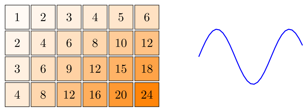
\usepackage{tikz}\begin{tikzpicture}
% a loop inside a loop: one cell for every pair (x, y)
\foreach \x in {1,...,6}
\foreach \y in {1,...,4} {
\pgfmathtruncatemacro{\p}{\x*\y}
\pgfmathtruncatemacro{\s}{4*\p}
\node[draw, minimum size=7mm, fill=orange!\s] at (0.75*\x, -0.75*\y) {\p};
}
% foreach inside a path: one -- step per value
\draw[thick, blue] (6,-1.9)
\foreach \x in {0.1,0.2,...,3} { -- (6+\x, {-1.9 + 0.8*sin(3*\x r)}) };
\end{tikzpicture}Full document
\documentclass[border=4pt]{standalone}
\usepackage{tikz}
\begin{document}
\begin{tikzpicture}
  % a loop inside a loop: one cell for every pair (x, y)
  \foreach \x in {1,...,6}
    \foreach \y in {1,...,4} {
      \pgfmathtruncatemacro{\p}{\x*\y}
      \pgfmathtruncatemacro{\s}{4*\p}
      \node[draw, minimum size=7mm, fill=orange!\s] at (0.75*\x, -0.75*\y) {\p};
    }
  % foreach inside a path: one -- step per value
  \draw[thick, blue] (6,-1.9)
    \foreach \x in {0.1,0.2,...,3} { -- (6+\x, {-1.9 + 0.8*sin(3*\x r)}) };
\end{tikzpicture}
\end{document}Scopes: grouping options and transformations
\begin{scope}[options] … \end{scope} applies its options to everything inside and nothing outside: colours, line styles, every node/.style, and transformations such as shift={(2,1)}, xshift=2cm, rotate=20 and scale=1.5. The same code inside differently transformed scopes draws moved, turned or resized copies. Transformations move and scale coordinates, not line widths, and nodes keep their size and orientation unless you add transform shape.
With \usetikzlibrary{scopes}, a brace followed by options, {[red] \draw …; }, is a shorter way to write a scope inside a picture. Options in the tikzpicture brackets act as a scope for the whole picture.
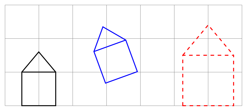
\usepackage{tikz}\begin{tikzpicture}
\draw[help lines] (0,0) grid (7,3);
% options on a scope apply to everything inside it
\begin{scope}[thick]
\draw (0.5,0) rectangle (1.5,1) (0.5,1) -- (1,1.6) -- (1.5,1);
\end{scope}
% the same code, moved to a new origin and turned
\begin{scope}[shift={(2.5,0.5)}, rotate=20, thick, blue]
\draw (0.5,0) rectangle (1.5,1) (0.5,1) -- (1,1.6) -- (1.5,1);
\end{scope}
% scaled: positions grow, the line width does not
\begin{scope}[shift={(4.5,0)}, scale=1.5, thick, red, dashed]
\draw (0.5,0) rectangle (1.5,1) (0.5,1) -- (1,1.6) -- (1.5,1);
\end{scope}
\end{tikzpicture}Full document
\documentclass[border=4pt]{standalone}
\usepackage{tikz}
\begin{document}
\begin{tikzpicture}
  \draw[help lines] (0,0) grid (7,3);
  % options on a scope apply to everything inside it
  \begin{scope}[thick]
    \draw (0.5,0) rectangle (1.5,1) (0.5,1) -- (1,1.6) -- (1.5,1);
  \end{scope}
  % the same code, moved to a new origin and turned
  \begin{scope}[shift={(2.5,0.5)}, rotate=20, thick, blue]
    \draw (0.5,0) rectangle (1.5,1) (0.5,1) -- (1,1.6) -- (1.5,1);
  \end{scope}
  % scaled: positions grow, the line width does not
  \begin{scope}[shift={(4.5,0)}, scale=1.5, thick, red, dashed]
    \draw (0.5,0) rectangle (1.5,1) (0.5,1) -- (1,1.6) -- (1.5,1);
  \end{scope}
\end{tikzpicture}
\end{document}Styles with \tikzset: /.style, /.append style and parameters
A style is a named list of options. \tikzset{box/.style={draw, rounded corners}} in the preamble defines it for the whole document; the same box/.style={…} in the options of a picture or scope defines it only there. Then \node[box] {…}; uses it, and changing the style changes every node at once.
- Parameters:
#1in a style is replaced by the value: withbox/.style={draw, fill=#1!15},box=redgives a light red fill.box/.default=bluesets the value used when you write justbox; without a default,#1is empty, which here would make the fill colour!15and stop with an undefined colour. - Two parameters:
tag/.style 2 args={fill=#1, text=#2}, used astag={black}{white}. - Adding to a style:
box/.append style={thick}adds options at the end (later options win),/.prefix styleat the beginning. This is how you change built-in styles:help lines/.append style={blue!50},every node/.append style={font=\small}. - Every-styles:
every node,every path,every pictureand others are applied automatically, so\tikzset{every picture/.style={thick}}changes all pictures.
The older form \tikzstyle{box}=[draw] still compiles but is no longer described in the current manual; use \tikzset.
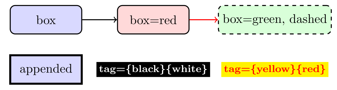
\usepackage{tikz}\tikzset{
box/.style={draw, thick, rounded corners, fill=#1!15, minimum width=20mm, minimum height=8mm},
box/.default=blue,
tag/.style 2 args={fill=#1, text=#2, font=\footnotesize\bfseries, inner sep=2pt},
}
\begin{tikzpicture}[link/.style={->, thick, #1}, link/.default=black]
\node[box] (a) at (0,0) {box};
\node[box=red] (b) at (3,0) {box=red};
\node[box=green, dashed] (c) at (6.4,0) {box=green, dashed};
\draw[link] (a) -- (b);
\draw[link=red] (b) -- (c);
% append options to a style, here only inside the scope
\begin{scope}[box/.append style={ultra thick, sharp corners}]
\node[box] at (0,-1.4) {appended};
\end{scope}
\node[tag={black}{white}] at (3,-1.4) {tag=\{black\}\{white\}};
\node[tag={yellow}{red}] at (6.4,-1.4) {tag=\{yellow\}\{red\}};
\end{tikzpicture}Full document
\documentclass[border=4pt]{standalone}
\usepackage{tikz}
\begin{document}
\tikzset{
  box/.style={draw, thick, rounded corners, fill=#1!15, minimum width=20mm, minimum height=8mm},
  box/.default=blue,
  tag/.style 2 args={fill=#1, text=#2, font=\footnotesize\bfseries, inner sep=2pt},
}
\begin{tikzpicture}[link/.style={->, thick, #1}, link/.default=black]
  \node[box] (a) at (0,0) {box};
  \node[box=red] (b) at (3,0) {box=red};
  \node[box=green, dashed] (c) at (6.4,0) {box=green, dashed};
  \draw[link] (a) -- (b);
  \draw[link=red] (b) -- (c);
  % append options to a style, here only inside the scope
  \begin{scope}[box/.append style={ultra thick, sharp corners}]
    \node[box] at (0,-1.4) {appended};
  \end{scope}
  \node[tag={black}{white}] at (3,-1.4) {tag=\{black\}\{white\}};
  \node[tag={yellow}{red}] at (6.4,-1.4) {tag=\{yellow\}\{red\}};
\end{tikzpicture}
\end{document}Decorations: zigzags, coils, random steps and braces
A decoration replaces a path by a changed version of it. Load the library family you need, then add decorate and a decoration={name, options} to the path; decoration alone only chooses the decoration and draws nothing different. decorations.pathmorphing bends the path (zigzag, snake, coil, bumps, saw, random steps), with amplitude and segment length as the main options. decorations.pathreplacing replaces it, most often by a curly brace (with mirror for the other side and raise to lift it off the path).
random steps changes on every compilation unless you fix the seed with \pgfmathsetseed{…}. pre length and post length leave the start and end of a path undecorated, useful for springs and wires. On very long paths, decorations can stop with Dimension too large; the decorations chapter of the manual has a section on handling that error.
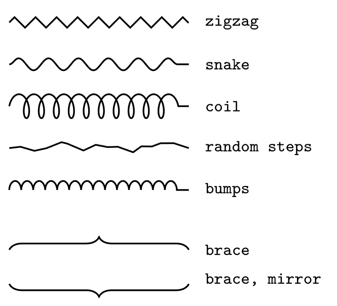
\usepackage{tikz} \usetikzlibrary{decorations.pathmorphing} \usetikzlibrary{decorations.pathreplacing}\begin{tikzpicture}[thick, every node/.style={right=4pt, font=\footnotesize\ttfamily}]
\pgfmathsetseed{7} % the same random steps on every run
\draw[decorate, decoration=zigzag] (0,0) -- (3,0) node {zigzag};
\draw[decorate, decoration={snake, amplitude=1mm, segment length=5mm}]
(0,-0.7) -- (3,-0.7) node {snake};
\draw[decorate, decoration={coil, aspect=0.5, amplitude=2mm, segment length=2.5mm}]
(0,-1.4) -- (3,-1.4) node {coil};
\draw[decorate, decoration={random steps, segment length=2mm, amplitude=1mm}]
(0,-2.1) -- (3,-2.1) node {random steps};
\draw[decorate, decoration={bumps, amplitude=1.5mm, segment length=4mm}]
(0,-2.8) -- (3,-2.8) node {bumps};
\draw[decorate, decoration={brace, amplitude=6pt}]
(0,-3.8) -- (3,-3.8) node {brace};
\draw[decorate, decoration={brace, amplitude=6pt, mirror, raise=2pt}]
(0,-4.3) -- (3,-4.3) node {brace, mirror};
\end{tikzpicture}Full document
\documentclass[border=4pt]{standalone}
\usepackage{tikz}
\usetikzlibrary{decorations.pathmorphing}
\usetikzlibrary{decorations.pathreplacing}
\begin{document}
\begin{tikzpicture}[thick, every node/.style={right=4pt, font=\footnotesize\ttfamily}]
  \pgfmathsetseed{7}  % the same random steps on every run
  \draw[decorate, decoration=zigzag] (0,0) -- (3,0) node {zigzag};
  \draw[decorate, decoration={snake, amplitude=1mm, segment length=5mm}]
    (0,-0.7) -- (3,-0.7) node {snake};
  \draw[decorate, decoration={coil, aspect=0.5, amplitude=2mm, segment length=2.5mm}]
    (0,-1.4) -- (3,-1.4) node {coil};
  \draw[decorate, decoration={random steps, segment length=2mm, amplitude=1mm}]
    (0,-2.1) -- (3,-2.1) node {random steps};
  \draw[decorate, decoration={bumps, amplitude=1.5mm, segment length=4mm}]
    (0,-2.8) -- (3,-2.8) node {bumps};
  \draw[decorate, decoration={brace, amplitude=6pt}]
    (0,-3.8) -- (3,-3.8) node {brace};
  \draw[decorate, decoration={brace, amplitude=6pt, mirror, raise=2pt}]
    (0,-4.3) -- (3,-4.3) node {brace, mirror};
\end{tikzpicture}
\end{document}Markings: arrows and symbols along a path
decorations.markings places arbitrary code at positions along a path without changing the path. It is normally used as a postaction, so the path is drawn first and then decorated: postaction={decorate}, decoration={markings, mark=at position 0.5 with {\arrow{Stealth}}} puts an arrow tip halfway. Positions are a fraction of the length (0.5), a distance from the start (1cm) or, when negative, a distance from the end (-1cm); mark=between positions 0.1 and 1 step 0.2 with {…} repeats the mark. Inside the mark, the origin is at the mark and the x axis points along the path, so \fill (0,0) circle (2pt); draws a dot on the path.
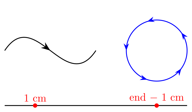
\usepackage{tikz} \usetikzlibrary{decorations.markings, arrows.meta}\begin{tikzpicture}[thick]
% one arrow tip halfway along a curve
\draw[postaction={decorate}, decoration={markings,
mark=at position 0.5 with {\arrow{Stealth[length=3mm]}}}]
(0,0) .. controls (1,1.5) and (2,-1.5) .. (3,0);
% a mark every fifth of the way round a circle
\draw[blue, postaction={decorate}, decoration={markings,
mark=between positions 0.1 and 1 step 0.2 with {\arrow{Stealth}}}]
(5,0) circle[radius=1];
% any drawing code at a distance along the path
\draw[postaction={decorate}, decoration={markings,
mark=at position 1cm with {\fill[red] (0,0) circle (2pt) node[above] {1 cm};},
mark=at position -1cm with {\fill[red] (0,0) circle (2pt) node[above] {end $-$ 1 cm};}}]
(0,-1.8) -- (6,-1.8);
\end{tikzpicture}Full document
\documentclass[border=4pt]{standalone}
\usepackage{tikz}
\usetikzlibrary{decorations.markings, arrows.meta}
\begin{document}
\begin{tikzpicture}[thick]
  % one arrow tip halfway along a curve
  \draw[postaction={decorate}, decoration={markings,
      mark=at position 0.5 with {\arrow{Stealth[length=3mm]}}}]
    (0,0) .. controls (1,1.5) and (2,-1.5) .. (3,0);
  % a mark every fifth of the way round a circle
  \draw[blue, postaction={decorate}, decoration={markings,
      mark=between positions 0.1 and 1 step 0.2 with {\arrow{Stealth}}}]
    (5,0) circle[radius=1];
  % any drawing code at a distance along the path
  \draw[postaction={decorate}, decoration={markings,
      mark=at position 1cm with {\fill[red] (0,0) circle (2pt) node[above] {1 cm};},
      mark=at position -1cm with {\fill[red] (0,0) circle (2pt) node[above] {end $-$ 1 cm};}}]
    (0,-1.8) -- (6,-1.8);
\end{tikzpicture}
\end{document}Grids and axes
\draw (0,0) grid (4,3); draws grid lines in the rectangle between the two corners, step apart (initially 1 cm); xstep and ystep set the two directions separately. The lines are placed at multiples of the step, counted from the origin, not from the first corner. A fine light grid under a coarser one and a pair of axes with ticks from \foreach make graph paper. help lines is the predefined grid style (black!50, very thin).
Rounding can drop the first or last line when a corner lies exactly on a multiple of the step: with xstep=0.5 from x = 6, our render lost the line at 6. The manual’s remedy is to move the corners slightly outwards, which is why the right-hand grid runs from (5.9,−0.1) to (8.1,3.1).
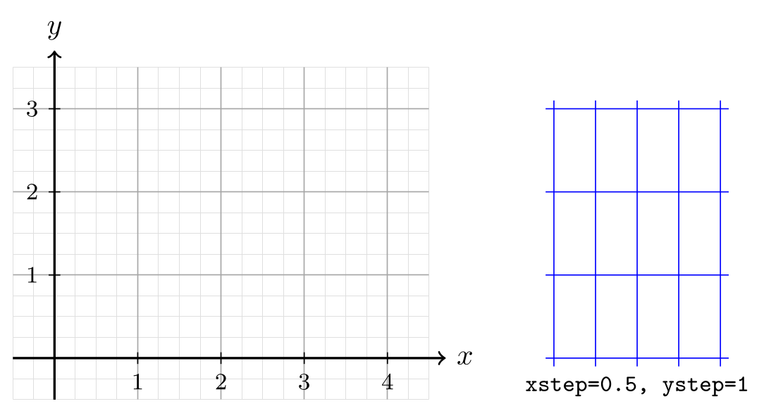
\usepackage{tikz}\begin{tikzpicture}
\draw[step=0.25, gray!25, very thin] (-0.5,-0.5) grid (4.5,3.5);
\draw[step=1, gray!70] (-0.5,-0.5) grid (4.5,3.5);
\draw[->, thick] (-0.5,0) -- (4.7,0) node[right] {$x$};
\draw[->, thick] (0,-0.5) -- (0,3.7) node[above] {$y$};
\foreach \x in {1,...,4}
\draw (\x,2pt) -- (\x,-2pt) node[below, font=\footnotesize] {\x};
\foreach \y in {1,...,3}
\draw (2pt,\y) -- (-2pt,\y) node[left, font=\footnotesize] {\y};
% different steps in x and y
\draw[blue, xstep=0.5, ystep=1] (5.9,-0.1) grid (8.1,3.1);
\node[below, font=\footnotesize\ttfamily] at (7,-0.1) {xstep=0.5, ystep=1};
\end{tikzpicture}Full document
\documentclass[border=4pt]{standalone}
\usepackage{tikz}
\begin{document}
\begin{tikzpicture}
  \draw[step=0.25, gray!25, very thin] (-0.5,-0.5) grid (4.5,3.5);
  \draw[step=1, gray!70] (-0.5,-0.5) grid (4.5,3.5);
  \draw[->, thick] (-0.5,0) -- (4.7,0) node[right] {$x$};
  \draw[->, thick] (0,-0.5) -- (0,3.7) node[above] {$y$};
  \foreach \x in {1,...,4}
    \draw (\x,2pt) -- (\x,-2pt) node[below, font=\footnotesize] {\x};
  \foreach \y in {1,...,3}
    \draw (2pt,\y) -- (-2pt,\y) node[left, font=\footnotesize] {\y};
  % different steps in x and y
  \draw[blue, xstep=0.5, ystep=1] (5.9,-0.1) grid (8.1,3.1);
  \node[below, font=\footnotesize\ttfamily] at (7,-0.1) {xstep=0.5, ystep=1};
\end{tikzpicture}
\end{document}Common errors and how to fix them
| LaTeX says (or you see) | Cause and fix |
|---|---|
| Package tikz Error: You need to say \usetikzlibrary{calc} for coordinate calculation. | Add \usetikzlibrary{calc} to the preamble; ($…$) coordinates need it. |
| Package pgfkeys Error: I do not know the key '/tikz/name path', to which you passed 'a', and I am going to ignore it. Perhaps you misspelled it. | name path and name intersections come from the intersections library: add \usetikzlibrary{intersections}. |
| Package tikz Error: You need to load a decoration library. | decorate with decoration=zigzag (or snake, coil, brace…) needs \usetikzlibrary{decorations.pathmorphing} or decorations.pathreplacing, decorations.markings, decorations.text. |
| Package tikz Error: Giving up on this path. Did you forget a semicolon? | Besides a missing ;, this appears when a coordinate contains parentheses, as in (1,sin(30)). Put the expression in braces: (1,{sin(30)}). |
| Paragraph ended before \pgffor@next was complete. | A \foreach without braces runs up to the next semicolon. Add the ; at the end of the command in the loop, or put the body in { }. |
| Package xcolor Error: Undefined color `'. | A style that uses #1 (for example fill=#1!20) was used without a value. Give it one (box=red) or set a default: box/.default=blue. |
| The last value of a \foreach range is missing | Fractional steps are rounded: {0,0.1,...,0.5} stops at 0.40002. End slightly higher ({0,0.1,...,0.501}) or loop over integers and divide. |
| The first or last line of a grid is missing | A rounding effect when a corner lies on a multiple of the step: move the corners slightly outwards, for example (5.9,-0.1) grid (8.1,3.1). |
Frequently asked questions
What is the difference between + and ++ in TikZ?
Both are relative to the previous point. ++(1,0) also makes the new point the current point, so the next step starts there; +(1,0) leaves the current point where it was, so several + steps in a row are all measured from the same point.
How do I get the midpoint between two points in TikZ?
Load \usetikzlibrary{calc} and write ($(A)!0.5!(B)$). Other fractions work the same way: ($(A)!0.25!(B)$) is a quarter of the way, and ($(A)!1cm!(B)$) is 1 cm from A towards B. On a line you are drawing, a node with midway (or pos=0.5) also sits halfway.
How do I write a for loop in TikZ?
Use \foreach: \foreach \x in {0,...,5} \draw (\x,0) circle (2pt); draws six circles. Use {0,0.5,...,3} for another step, \x/\y pairs for several variables, and [count=\i] to number the items. Put several commands in braces after the list.
How do I define a reusable style with \tikzset?
Write \tikzset{mybox/.style={draw, rounded corners, fill=blue!10}} in the preamble and use \node[mybox] {…};. Add a parameter with #1 (fill=#1) and a default with mybox/.default=blue; add options to an existing style with mybox/.append style={thick}.
What units do TikZ coordinates use?
Plain numbers are multiples of the x and y vectors, which are 1 cm by default, so (2,1) is 2 cm right and 1 cm up. Numbers with units, such as (2cm,10pt), are taken literally and are not affected by x= and y=, but scale= changes both.
How do I draw a curve through specific points in TikZ?
A Bézier curve, (a) .. controls (c) and (d) .. (b), passes through a and b but not through the control points c and d. To pass through several points, use plot[smooth] coordinates {(0,0) (1,1) (2,0)}, or chain to[out=…, in=…] segments that set the angle at each point.
References
- PGF/TikZ manual, §13.2 Coordinate Systems (canvas, xyz, polar, node)tikz.dev
- PGF/TikZ manual, §13.3 Coordinates at Intersectionstikz.dev
- PGF/TikZ manual, §13.4 Relative and Incremental Coordinatestikz.dev
- PGF/TikZ manual, §13.5 Coordinate Calculations (calc)tikz.dev
- PGF/TikZ manual, §14 Syntax for Path Specificationstikz.dev
- PGF/TikZ manual, §14.3 The Curve-To Operationtikz.dev
- PGF/TikZ manual, §14.13 The To Path Operationtikz.dev
- PGF/TikZ manual, §14.8 The Grid Operationtikz.dev
- PGF/TikZ manual, §88 Repeating Things: The Foreach Statementtikz.dev
- PGF/TikZ manual, §12.3 Using Scopes to Structure a Picturetikz.dev
- PGF/TikZ manual, §12.4.2 Using Styles to Manage How Pictures Looktikz.dev
- PGF/TikZ manual, §87.4.4 Defining Styles (pgfkeys)tikz.dev
- PGF/TikZ manual, §24 Decorated Pathstikz.dev
- PGF/TikZ manual, §50 Decoration Library (path morphing, replacing, markings)tikz.dev
- pgf package (TikZ) on CTAN, with the full manual as PDFctan.org
The facts on this page were checked against these sources, and every picture is the code with it typeset with TeX Live 2026. Code on this page: CC0 1.0, copy it freely.
Try the code in your browserEvery snippet on this page opens in the free TikZ editor: it is typeset with TeX Live as you type, with errors pointed at their line.
Open the TikZ editor