Cyclic voltammetry (CV): how it works and how to read a voltammogram
Cyclic voltammetry (CV) sweeps the potential of a working electrode linearly against a reference electrode, forward and then back, while recording the current; the resulting current–potential trace is the cyclic voltammogram (Rafiee et al. 2024). Oxidation and reduction peaks appear where a redox couple reacts, the midpoint of the two peaks gives its formal potential, and for a reversible, diffusion-controlled couple the peaks sit about 59/n mV apart (Rafiee et al. 2024; Venton & Cao 2020). For materials scientists CV reports redox potentials, reversibility, whether a species diffuses or is adsorbed, coupled chemical steps, catalytic currents and the electrochemically active surface area of electrocatalysts (Rafiee et al. 2024; Sharma et al. 2026).
Contents
Cyclic voltammetry (CV) at a glance
| Probe | A linear potential sweep of the working electrode against a reference electrode, forward to a switching potential and back (Rafiee et al. 2024) |
|---|---|
| Signal measured | Current vs applied potential: the cyclic voltammogram (Rafiee et al. 2024) |
| Main information | Formal potentials, reversibility, diffusion vs adsorption control, coupled chemical (EC) steps and catalytic (EC′) currents (Rafiee et al. 2024; Venton & Cao 2020) |
| Cell | Three electrodes: working electrode, reference (Ag/AgCl, Hg/HgO, Hg/Hg₂SO₄ or Hg/Hg₂Cl₂, chosen by electrolyte pH) and an inert counter electrode such as a graphite rod or Pt mesh or wire (Sharma et al. 2026) |
| Typical scan rate | Around 100 mV s⁻¹ in conventional CV; around 400 V s⁻¹ in fast-scan CV at microelectrodes (Venton & Cao 2020) |
| Reversible couple | Peak separation about 59/n mV, where n is the number of electrons transferred (Venton & Cao 2020) |
| Peak current | Randles–Ševčík: proportional to √v for a diffusing species (Rafiee et al. 2024); proportional to v for an adsorbed species (Venton & Cao 2020) |
| Potential scale in electrocatalysis | Reversible hydrogen electrode (RHE); OER E° = 1.23 V and HER E° = 0.00 V vs RHE (Sondermann et al. 2025) |
| Surface area from CV | Double-layer capacitance from CVs at several scan rates in a non-faradaic window; ECSA = Cdl / Cs with Cs = 0.04 mF cm⁻² in 1 M KOH (Sharma et al. 2026) |
Cyclic voltammetry (CV) instrument drawing (high-resolution SVG)
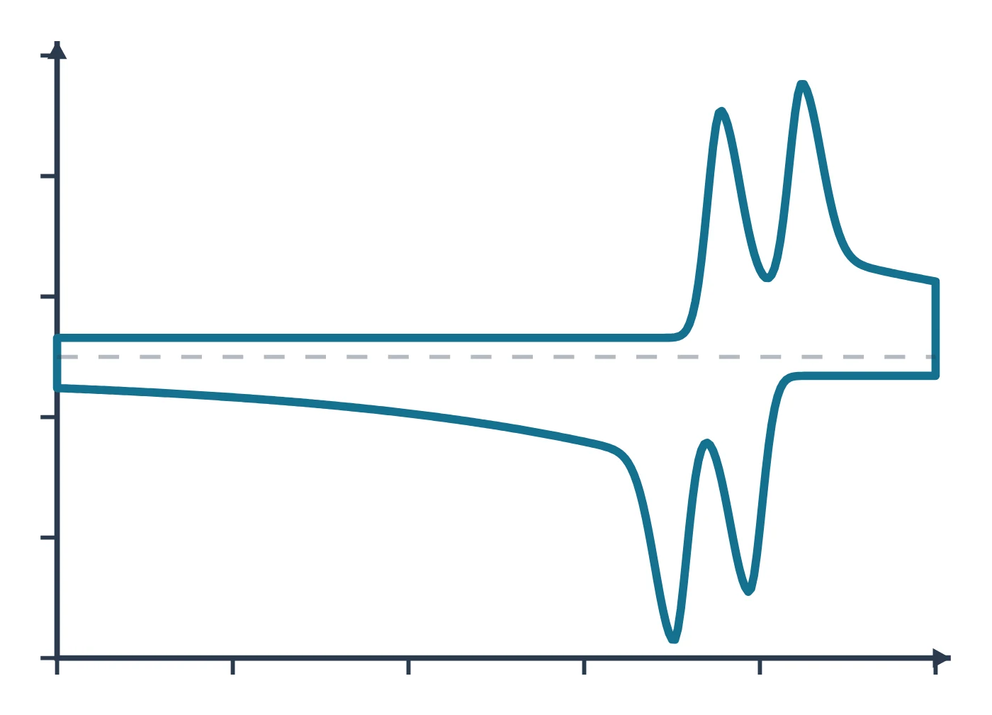
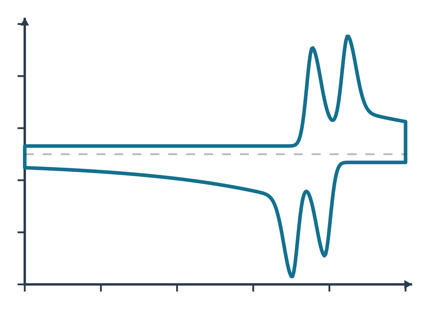
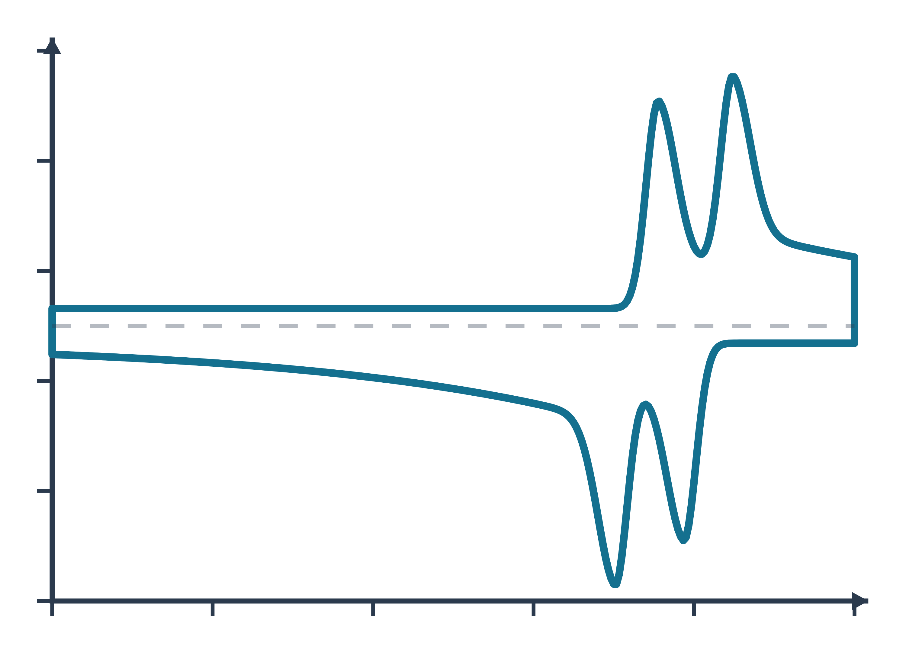
Cyclic voltammetry (CV) data: an example plot to edit
How CV works
A potentiostat controls the potential of the working electrode relative to a reference electrode and passes current through a counter electrode. In a CV experiment it scans that potential linearly from an initial value past the formal potential of the analyte to a switching potential, then reverses and scans back, usually to the starting value, while recording the current (Rafiee et al. 2024). If the solution contains the reduced form of a couple, the forward (anodic) scan oxidises it and the reverse (cathodic) scan reduces the product back (Rafiee et al. 2024).
The experiment is run in an unstirred, quiescent solution, so diffusion is the main way the analyte reaches the electrode. As the potential passes the formal potential the analyte near the surface is consumed, the diffusion layer grows and the current peaks and then decays, which gives the classic "duck" shape (Rafiee et al. 2024). The scan rate sets the time scale: the peak current rises with the square root of the scan rate for a diffusing species, as described by the Randles–Ševčík equation (Rafiee et al. 2024), which at 25 °C reads
iₚ = (2.69 × 10⁵) n³ᐟ² A D¹ᐟ² C v¹ᐟ²
with n the number of electrons, A the electrode area in cm², D the diffusion coefficient in cm² s⁻¹, C the concentration in mol cm⁻³ and v the scan rate in V s⁻¹ (Rafiee et al. 2024). For a species adsorbed on the electrode the current instead grows linearly with scan rate (Venton & Cao 2020). A one-way sweep without the return scan is linear sweep voltammetry (LSV), the standard way to record polarisation curves of electrocatalysts (Sharma et al. 2026).
Reference electrodes and the RHE scale. Aqueous work uses Ag/AgCl, Hg/HgO, Hg/Hg₂SO₄ or Hg/Hg₂Cl₂ references chosen by the pH of the electrolyte (Sharma et al. 2026). Because the thermodynamic potentials of the hydrogen and oxygen evolution reactions shift with pH, electrocatalysis papers convert every potential to the reversible hydrogen electrode (RHE) with the Nernst equation (Sharma et al. 2026):
E(RHE) = E(ref) + E°(ref) + 0.059 × pH
where 0.059 V is the Nernst factor at 298 K and E°(ref) is the standard potential of the reference, 0.0983 V for Hg/HgO in saturated 1 M NaOH (Sharma et al. 2026). In 1 M KOH (pH 14) a reading against Hg/HgO therefore moves up by about 0.924 V (calculated from 0.0983 + 0.059 × 14). On the RHE scale the OER has E° = 1.23 V and the HER 0.00 V, and the overpotential is the measured, iR-corrected potential minus 1.23 V (Sondermann et al. 2025). The free LabCanvas RHE calculator does this conversion for common reference electrodes and any pH.
What the data looks like and how to read it
- Peak potentials. A CV has an anodic and a cathodic peak potential; for well-behaved couples their midpoint (E½) coincides with the formal potential E°′ (Rafiee et al. 2024).
- Peak separation and reversibility. A reversible, diffusion-controlled couple shows a peak separation of about 59/n mV (Venton & Cao 2020). Wider separations mean slower electron transfer: dopamine at glassy carbon gives 70 mV at conventional scan rates, so it is not reversible, and at 400 V s⁻¹ the separation reaches about 750 mV (Venton & Cao 2020). A surface-bound (adsorbed) species ideally gives 0 mV separation and symmetric peaks (Venton & Cao 2020).
- Scan-rate test. Record CVs at several scan rates: current proportional to √v points to diffusion, current proportional to v to adsorption (Rafiee et al. 2024; Venton & Cao 2020). Dividing the current by √v lets CVs at different scan rates be overlaid, which shows mechanistic changes clearly (Rafiee et al. 2024).
- Coupled chemistry. If the electrogenerated species reacts (an EC mechanism) the return peak shrinks, so the reverse-to-forward peak-current ratio falls below one, and it rises again at faster scans (Rafiee et al. 2024).
- Catalysis. When a mediator or electrocatalyst is regenerated by a substrate (EC′), the forward current grows into a sigmoidal wave with a scan-rate-independent plateau whose height reflects the catalytic turnover rate, and the return peak disappears (Rafiee et al. 2024).
- Electrocatalyst CVs. Ni-based OER catalysts show a Ni²⁺/Ni³⁺ oxidation peak around 1.35–1.45 V vs RHE before oxygen evolution starts (Beglau et al. 2023), and the overpotential at 10 mA cm⁻² is read from the LSV (Sharma et al. 2026).
- Tafel plots. Plotting overpotential against log current density gives η = a + b log j; the slope b, in mV dec⁻¹, is the extra overpotential needed to raise the current tenfold (Beglau et al. 2023; Sharma et al. 2026). The LabCanvas Tafel slope calculator fits the linear region of your own η–log j data.
Sample preparation
- Molecular solutions. Record molecular analytes in an unstirred solution so that mass transport is by diffusion (Rafiee et al. 2024).
- Remove oxygen. Purging the electrolyte with nitrogen for about 10 min before measuring removes dissolved O₂ (Beglau et al. 2023; Sondermann et al. 2025).
- Catalyst inks. A typical OER protocol drops 10 µL of catalyst ink onto a rotating disc electrode of 0.196 cm² (0.25 mg cm⁻²), rotates it at 1600 rpm and pre-cycles until the response is steady (Beglau et al. 2023); powders can also be coated onto carbon paper and activated by 10 cycles between 1.0 and 1.7 V vs RHE at 100 mV s⁻¹ (Sondermann et al. 2025).
- Loading and substrate. Report the mass loading: for NiO on carbon cloth the overpotential fell as loading rose from 0.2 to 0.6 mg cm⁻² (Sharma et al. 2026). The support matters too: nickel foam gives far higher currents than carbon cloth and adds its own Ni redox peak (Sharma et al. 2026).
- Uncompensated resistance. Measure the electrolyte resistance Rₛ by EIS, for example at open-circuit potential, and correct the potential for iR drop (Beglau et al. 2023; Sharma et al. 2026).
What CV tells you about materials
Redox thermodynamics. Redox potentials from CV are quick to measure and correlate with thermodynamic quantities such as substituent effects and catalyst reactivity, which is why they guide the design of mediators and catalysts (Rafiee et al. 2024).
Electrocatalysts for water splitting. LSV and CV give onset potentials, overpotentials at a set current density, Tafel slopes and stability over 1000 or more cycles (Sharma et al. 2026). Metal–organic frameworks are widely tested this way as OER (pre-)catalysts: a NiFe MOF/carbon nanotube composite reached 301 mV at 10 mA cm⁻² with a Tafel slope of 58 mV dec⁻¹ against 354 mV and 91 mV dec⁻¹ for RuO₂ (Sondermann et al. 2025), and Ni(Fe) MOFs transform during OER into Ni(OH)₂, NiOOH and FeOOH phases (Beglau et al. 2023). For the frameworks themselves see our pages on HKUST-1, ZIF-8 and UiO-66.
Active surface area and active sites. CVs in a potential window without faradaic reactions measure the double-layer capacitance: half the slope of Δj against scan rate gives Cdl, and dividing by a specific capacitance (0.04 mF cm⁻² in 1 M KOH, 0.035 mF cm⁻² in 1 M H₂SO₄) gives the ECSA (Sharma et al. 2026). For Pt, hydrogen underpotential deposition or CO stripping (420 µC cm⁻²) counts surface sites, and for transition-metal catalysts integrating a redox peak counts the metal sites that switch oxidation state (Sharma et al. 2026). Compare the ECSA with the gas-adsorption area from BET, and the surface oxidation states with XPS.
CV and electrochemical impedance spectroscopy are usually run in the same cell; both are part of our guide to characterisation techniques.
Common mistakes and limits
- Scanning too fast for activity metrics. Faster LSV scans add capacitive current and make catalysts look better: on carbon cloth the overpotential at 10 mA cm⁻² dropped from 796 mV at 1 mV s⁻¹ to 647 mV at 25 mV s⁻¹, an 18.71% error, so the authors recommend ≤2 mV s⁻¹ (Sharma et al. 2026). Charging current grows linearly with scan rate (Venton & Cao 2020).
- Trusting automatic iR compensation. Instrument-applied compensation did not match manual 100% correction, and on an electrode with Rₛ = 7 Ω full compensation distorted the curve, so only about 20% could be applied (Sharma et al. 2026). Report data with and without correction.
- Counting redox current as catalysis. A metal oxidation peak on the forward scan inflates OER current; the reverse scan gives activity free of it (Sharma et al. 2026).
- Over-reading Tafel slopes. Slopes from LSV or CV include double-layer and metal-redox current, different methods gave 59 to 82 mV dec⁻¹ for the same nickel foam, and steady-state chronoamperometry or chronopotentiometry is preferred (Sharma et al. 2026). The value also depends on the fitted range, and a Tafel slope alone does not prove one catalyst better than another (Sondermann et al. 2025).
- Mixing potential scales. Quote the reference electrode and convert to RHE with the electrolyte pH before comparing with other work (Sharma et al. 2026).
- ECSA window. Cdl depends on which non-faradaic window is chosen, and Ni-based hydroxides are not conductive below the Ni²⁺ oxidation, so impedance at OER potentials can be more reliable (Sharma et al. 2026).
- Stability from CV alone. 1000 CV cycles show on–off stability, but chronoamperometry or chronopotentiometry is preferred for claiming practical durability (Sharma et al. 2026).
How to draw the CV setup and data in LabCanvas
The LabCanvas figure editor Library has the potentiostat and three-electrode cell as an editable object, including a cutaway view of the cell that shows the working, reference and counter electrodes and the current path, plus an editable data plot for the voltammogram. Draw the forward and reverse scans with arrows, label the anodic and cathodic peaks, E½ and ΔEp, and state the reference electrode or RHE on the potential axis. Overlay CVs at several scan rates or before and after cycling, then export the panel for a methods figure, SI or graphical abstract.
CV compared with LSV, chronoamperometry and EIS
| Technique | Perturbation | Signal | Main use |
|---|---|---|---|
| Cyclic voltammetry (CV) | Linear potential sweep forward and back | Current vs potential | Redox potentials, reversibility, mechanisms, ECSA, cycling stability |
| Linear sweep voltammetry (LSV) | One-way linear sweep | Polarisation curve | Onset and overpotential of electrocatalysts; Tafel plots (slow scans) |
| Chronoamperometry (CA) | Potential step, then hold | Current vs time | Diffusion (Cottrell), kinetics, steady-state Tafel data, long-term stability |
| EIS | Small sinusoidal potential over many frequencies | Impedance vs frequency | Solution and charge-transfer resistance, capacitance, diffusion |
Related techniques
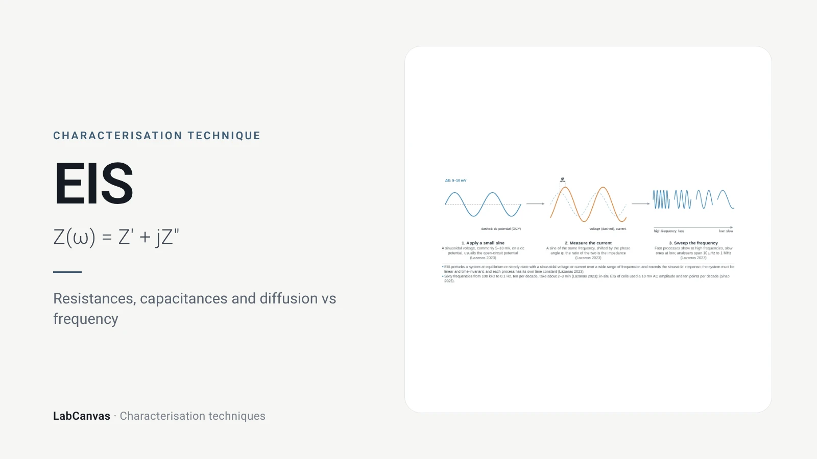
Electrochemical impedance spectroscopy (EIS)
EIS explained: small AC perturbation, Nyquist and Bode plots, Randles circuit, charge-transfer resistance, Warburg diffusion, batteries and catalysts.
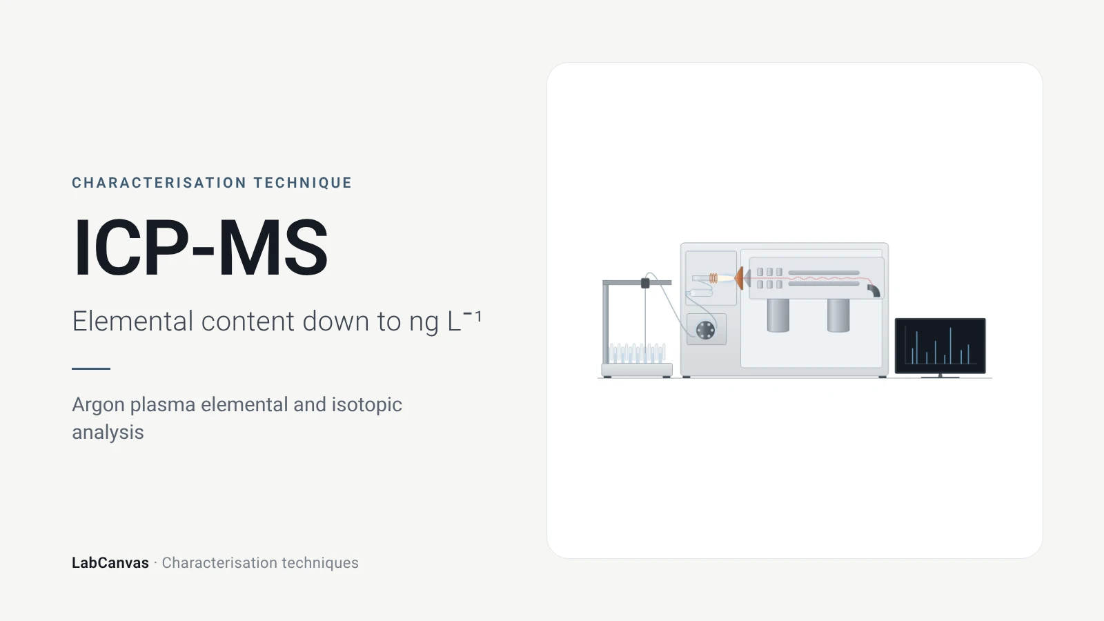
ICP-MS and ICP-OES
ICP-MS and ICP-OES explained: argon plasma, detection limits, acid digestion, interferences, single-particle ICP-MS and metal content of MOFs.
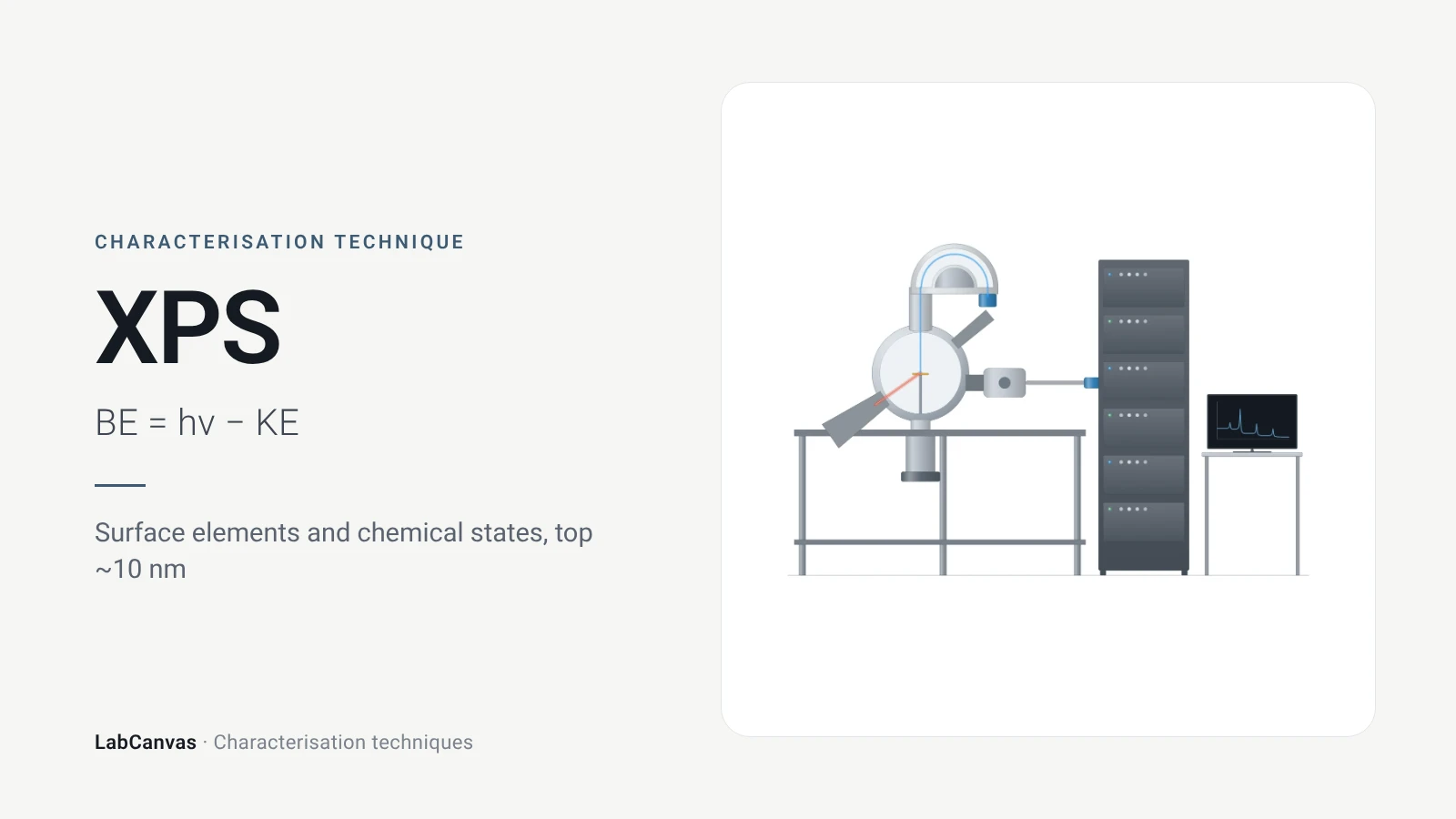
X-ray photoelectron spectroscopy (XPS)
XPS explained: binding energy, 2–10 nm surface sensitivity, survey vs high-resolution spectra, chemical shifts, C 1s charge referencing and depth profiling.
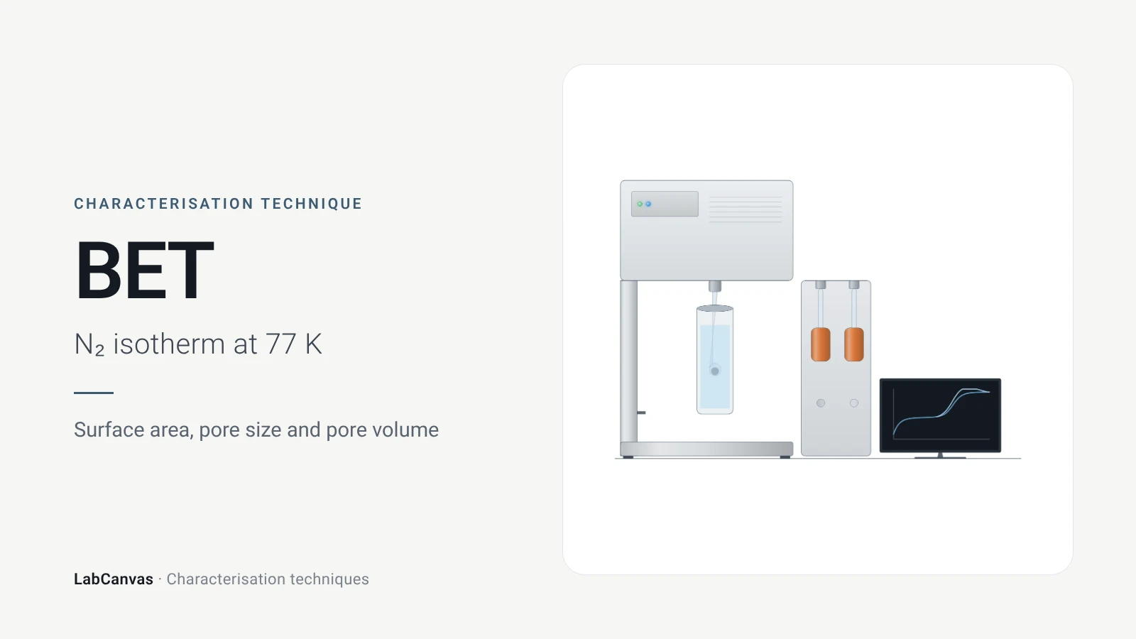
Gas sorption and BET surface area
BET surface area explained: N₂ sorption at 77 K, IUPAC isotherm types, the BET range and Rouquerol criteria, pore size, degassing and limits for MOFs.
More on LabCanvas
- All characterisation techniques: XRD, XPS, BET, SEM, TEM, NMR, FTIR, Raman and more, explained with cited sources
- Graphical abstract sizes and templates: ACS, Wiley, Angewandte, RSC, Elsevier and Cell Press, with templates at the right size
- RHE potential calculator: Free tool
- Tafel slope calculator: Free tool
- Materials explained: MOFs, COFs, 2D materials, perovskites, batteries and zeolites, with cited facts
- Journal figure size guide: Column widths and resolutions for 38 journals
Frequently asked questions
What is cyclic voltammetry used for?
CV measures current while the electrode potential is swept forward and back, revealing redox potentials, reversibility and coupled chemical reactions (Rafiee et al. 2024). In materials work it is also used to test electrocatalysts, estimate the electrochemically active surface area and check cycling stability (Sharma et al. 2026).
How do you read a cyclic voltammogram?
Find the anodic and cathodic peaks: their midpoint gives the formal potential, their separation tells you about reversibility and their currents scale with concentration (Rafiee et al. 2024; Venton & Cao 2020). A missing or shrinking return peak indicates a chemical step after electron transfer (Rafiee et al. 2024).
What peak separation means a reversible CV?
About 59/n mV, where n is the number of electrons transferred, for a reversible, diffusion-controlled couple (Venton & Cao 2020). Larger separations indicate slower electron transfer; an ideal adsorbed species shows 0 mV.
What is the Randles–Ševčík equation?
It gives the CV peak current of a diffusing species: at 25 °C, iₚ = 2.69 × 10⁵ n³ᐟ² A D¹ᐟ² C v¹ᐟ², so the peak current is proportional to the square root of the scan rate (Rafiee et al. 2024). A linear dependence on v instead points to an adsorbed species (Venton & Cao 2020).
How do you convert a potential to the RHE scale?
Use E(RHE) = E(ref) + E°(ref) + 0.059 × pH, with E°(ref) the standard potential of your reference electrode, for example 0.0983 V for Hg/HgO (Sharma et al. 2026). The free LabCanvas RHE calculator at /tools/rhe-calculator does the arithmetic.
What scan rate should I use for CV?
Conventional CV is run around 100 mV s⁻¹ (Venton & Cao 2020), and varying the scan rate tests diffusion vs adsorption (Rafiee et al. 2024). For electrocatalyst activity, LSV at 2 mV s⁻¹ or slower avoids overestimating current with capacitive charging (Sharma et al. 2026).
CV vs LSV: what is the difference?
LSV sweeps the potential in one direction only, while CV reverses the sweep and records the return scan, which shows whether the product can be converted back (Rafiee et al. 2024; Sharma et al. 2026). LSV is the usual way to report electrocatalyst overpotentials.
How is ECSA measured with cyclic voltammetry?
Record CVs at several scan rates in a potential window without faradaic reactions, plot the current-density difference against scan rate, take half the slope as the double-layer capacitance and divide by a specific capacitance such as 0.04 mF cm⁻² in 1 M KOH (Sharma et al. 2026).
References
- M. Rafiee, D. J. Abrams, L. Cardinale, Z. Goss, A. Romero-Arenas, S. S. Stahl. Cyclic voltammetry and chronoamperometry: mechanistic tools for organic electrosynthesis. Chem. Soc. Rev. 2024, 53, 566–585. doi:10.1039/d2cs00706a
- B. J. Venton, Q. Cao. Fundamentals of fast-scan cyclic voltammetry for dopamine detection. Analyst 2020, 145, 1158–1168. doi:10.1039/c9an01586h
- M. Sharma, C. Prakash, V. K. Singh, A. Dixit. A tutorial on measurement of electrochemical water-splitting performance parameters: methods and best practices. ACS Meas. Sci. Au 2026, 6, 1445–1470. doi:10.1021/acsmeasuresciau.6c00147
- L. Sondermann, L. M. Voggenauer, A. Vollrath, T. Strothmann, C. Janiak. Comparison of in situ and postsynthetic formation of MOF-carbon composites as electrocatalysts for the alkaline oxygen evolution reaction (OER). Molecules 2025, 30, 208. doi:10.3390/molecules30020208
- T. H. Y. Beglau, L. Rademacher, R. Oestreich, C. Janiak. Synthesis of Ketjenblack decorated pillared Ni(Fe) metal-organic frameworks as precursor electrocatalysts for enhancing the oxygen evolution reaction. Molecules 2023, 28, 4464. doi:10.3390/molecules28114464
Draw Cyclic voltammetry (CV) figures for your paper
LabCanvas is a browser workspace for scientific figures: instruments with their beam and light paths, editable data plots, crystal structures, graphs and graphical abstracts at journal sizes.
Draw Cyclic voltammetry (CV) in LabCanvas