Electrochemical impedance spectroscopy (EIS): principle, Nyquist plots and equivalent circuits
Electrochemical impedance spectroscopy (EIS) applies a small sinusoidal voltage (or current), usually on top of a DC potential, to an electrochemical cell over a wide range of frequencies and measures the impedance from the amplitude and phase of the response (Lazanas & Prodromidis 2023). Because double-layer charging, electron transfer and diffusion have different time constants, they appear at different frequencies and can be separated, typically by fitting an equivalent circuit such as the Randles circuit (Lazanas & Prodromidis 2023; Sharma et al. 2026). EIS gives a materials scientist the electrolyte resistance, charge-transfer resistance, double-layer capacitance and diffusion behaviour of batteries, electrocatalysts, solid electrolytes and sensors (Lazanas & Prodromidis 2023).
Contents
Electrochemical impedance spectroscopy (EIS) at a glance
| Probe | A small-amplitude sinusoidal voltage or current, usually superimposed on a DC signal, applied over a wide frequency range (Lazanas & Prodromidis 2023) |
|---|---|
| Signal measured | Impedance at each frequency: real part Z′, imaginary part Z″, modulus |Z| and phase (Lazanas & Prodromidis 2023) |
| Main information | Electrolyte (uncompensated) resistance, charge-transfer resistance, double-layer capacitance and diffusion (Lazanas & Prodromidis 2023) |
| Perturbation amplitude | 5–10 mV under potentiostatic control (Lazanas & Prodromidis 2023); 1, 2, 5 and 10 mV gave practically the same spectra on catalyst electrodes (Sharma et al. 2026) |
| Frequency range | Analysers span 10 µHz–1 MHz; the practical low limit is about 1 mHz, often 10–100 mHz (Lazanas & Prodromidis 2023) |
| High-frequency limit | Electrolyte resistance is reached at ca. 100 kHz in common cells; bulk ionic conduction in solid electrolytes needs >5 MHz (Lazanas & Prodromidis 2023) |
| Standard model | Randles circuit: solution resistance in series with the double-layer capacitance in parallel with charge-transfer resistance plus Warburg impedance (Lazanas & Prodromidis 2023) |
| Data check | Lissajous plots for linearity and stability; Kramers–Kronig test before fitting (Lazanas & Prodromidis 2023) |
| Example result | Rct of 7 Ω for a NiFe MOF–carbon nanotube OER catalyst vs 39 Ω for RuO₂, at 1.5 V vs RHE, 0.01 Hz–10 kHz, 10 mV (Sondermann et al. 2025) |
Electrochemical impedance spectroscopy (EIS) instrument drawing (high-resolution SVG)
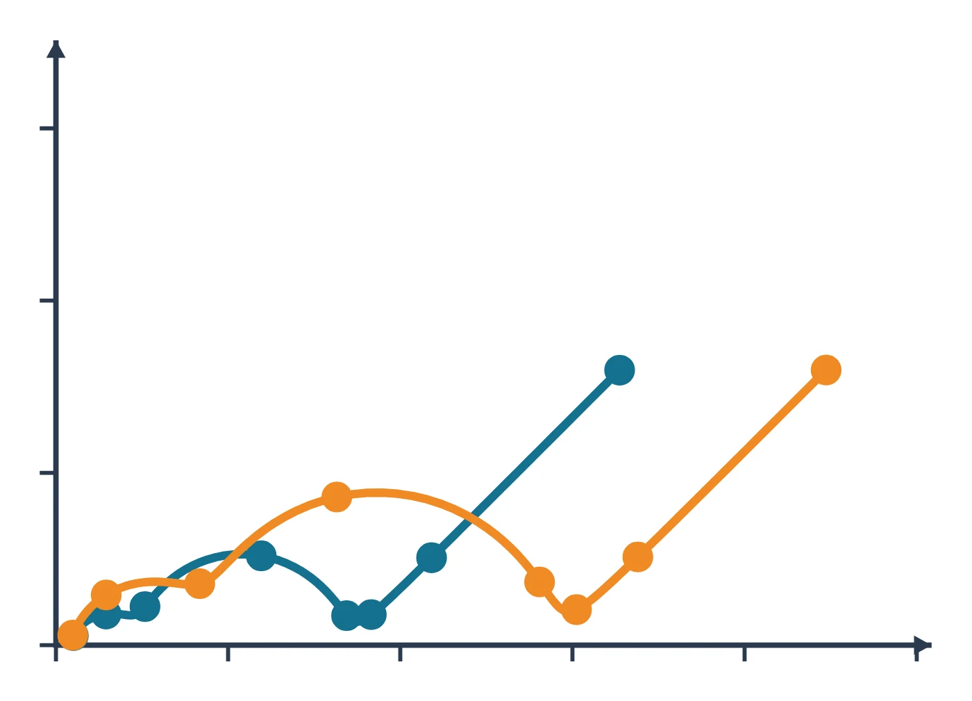
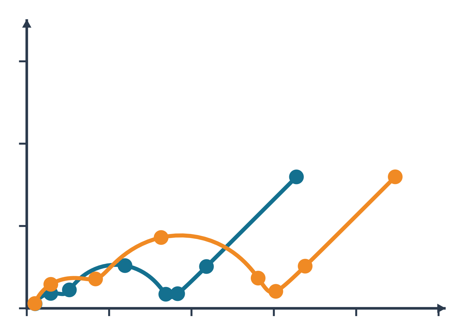
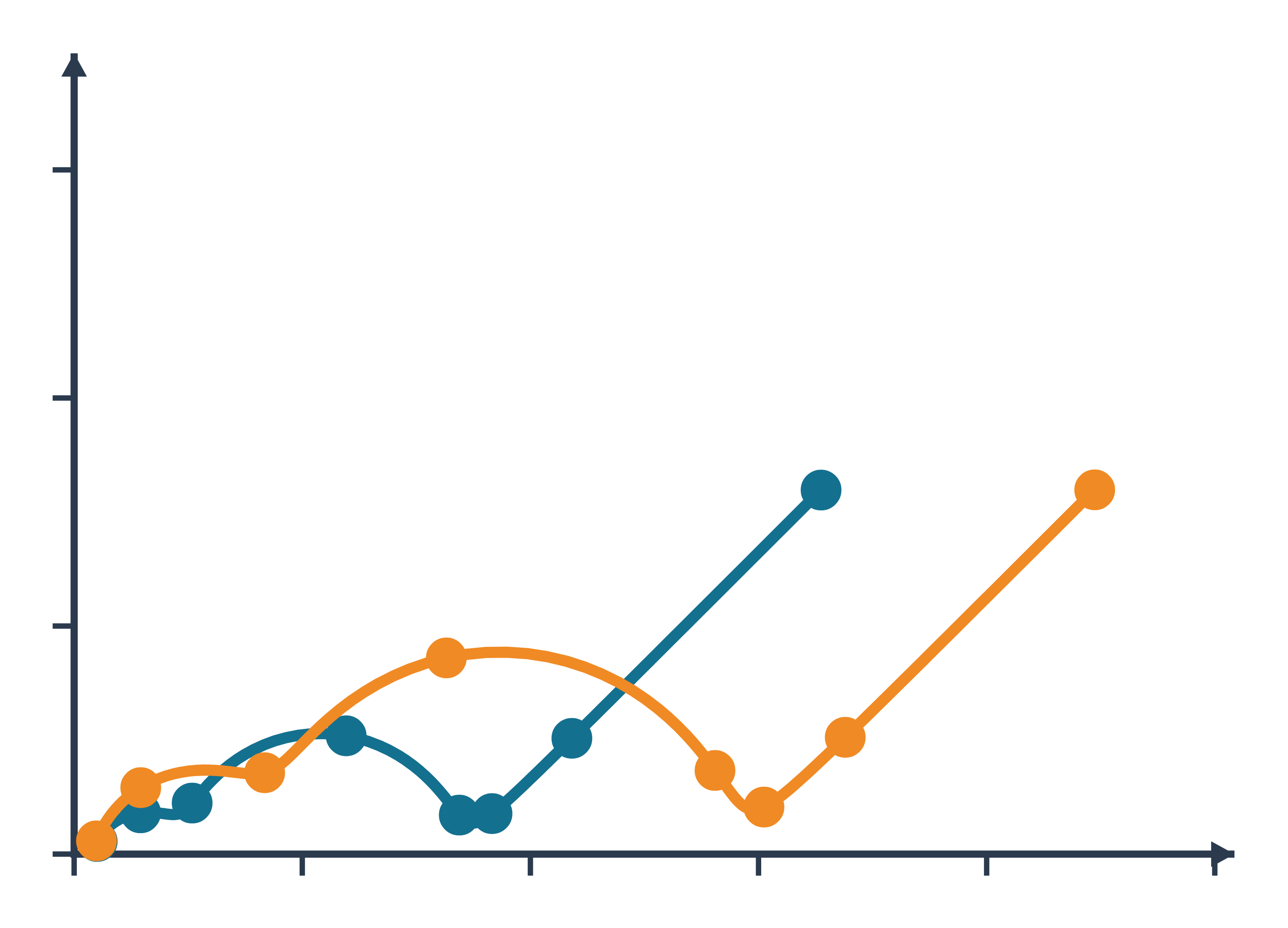
Electrochemical impedance spectroscopy (EIS) data: an example plot to edit
How EIS works
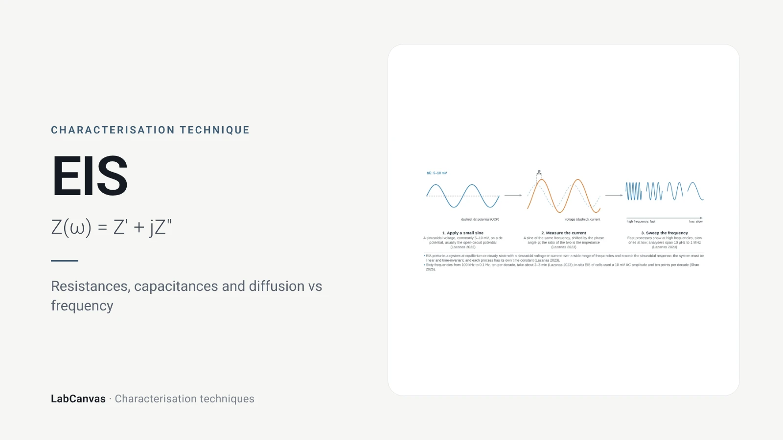
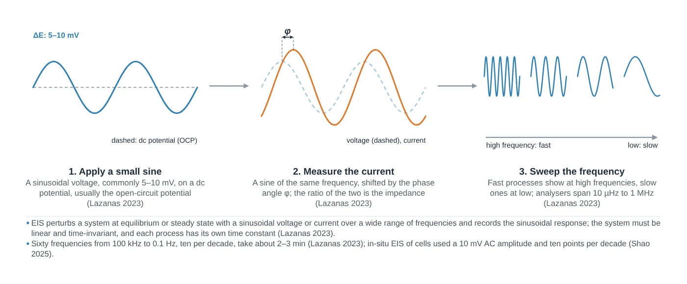
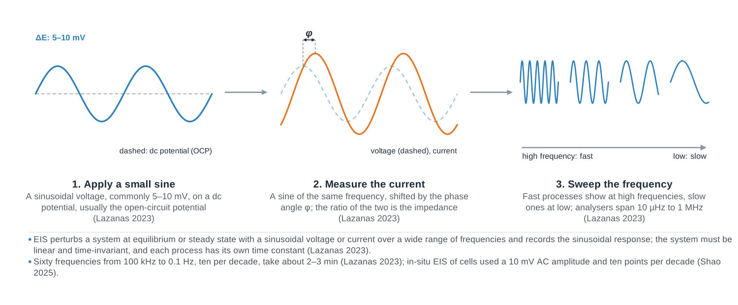
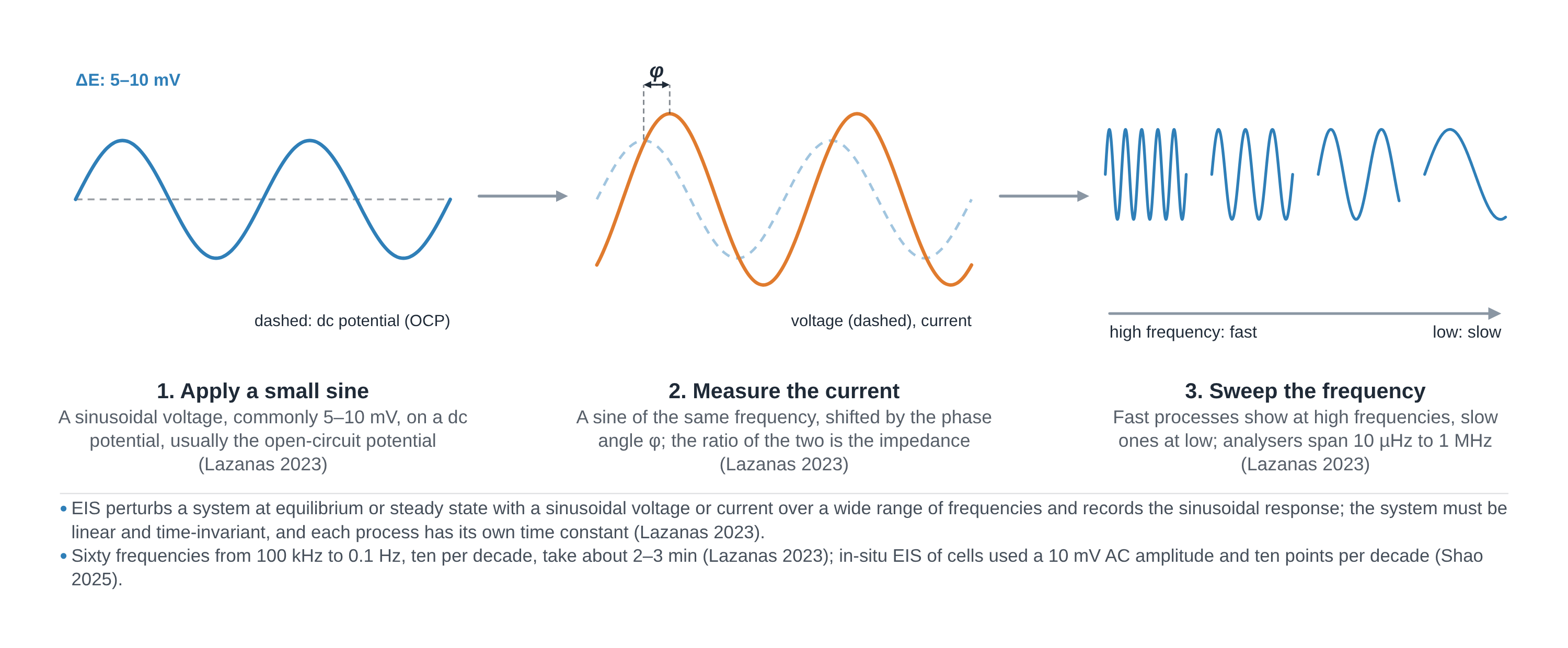
In EIS the potentiostat applies a small sinusoidal perturbation, normally a voltage of a few millivolts on top of a DC potential, and measures the current that flows at the same frequency; their ratio and phase shift give the impedance Z(ω) = Z′ + jZ″ at that frequency (Lazanas & Prodromidis 2023). The measurement is repeated across a wide frequency range, typically from some mHz to about 1 MHz (Lazanas & Prodromidis 2023).
The perturbation must be small because real electrochemical cells are not linear: only a small signal keeps the response linear, so that the output is a sinusoid of the same frequency and the impedance does not depend on the amplitude (Lazanas & Prodromidis 2023; Sharma et al. 2026). The cell must also stay unchanged during the sweep (Lazanas & Prodromidis 2023).
The power of EIS is that processes with different time constants respond at different frequencies: high frequencies probe fast processes and low frequencies slow ones (Sharma et al. 2026). In a worked example the double-layer charging, the faradaic reaction and diffusion had characteristic frequencies of 4.1 kHz, 310 Hz and 0.4 Hz, so a sweep from 10 kHz to 10 mHz covered all three (Lazanas & Prodromidis 2023). The cost is time: a single period at 1 mHz lasts 1000 s (calculated from 1/f), and at 10 µHz one measurement takes 27.8 h (Lazanas & Prodromidis 2023).
Equivalent circuits. Spectra are interpreted by fitting circuits of resistors, capacitors and distributed elements (Sharma et al. 2026). The Randles circuit puts the solution resistance Rₛ in series with the double-layer capacitance Cdl, which sits in parallel with the charge-transfer resistance Rct and the Warburg impedance Zw that describes diffusion of the redox species (Lazanas & Prodromidis 2023). Real, rough electrodes give depressed arcs that are fitted with a constant phase element (CPE) in place of the capacitor; its exponent n is 1 for an ideal capacitor, 0.5 for a Warburg element and 0 for a resistor (Lazanas & Prodromidis 2023).
What the data looks like and how to read it
- Nyquist plot. −Z″ is plotted against Z′, one point per frequency, with high frequencies on the left; both axes should have the same range (Lazanas & Prodromidis 2023). A resistor and capacitor in parallel give a semicircle whose diameter equals the resistance (Lazanas & Prodromidis 2023).
- Reading a Randles spectrum. The semicircle meets the real axis at Rₛ on the high-frequency side and at Rₛ + Rct on the low-frequency side, so its width is the charge-transfer resistance; this region is controlled by electron transfer (Lazanas & Prodromidis 2023). At lower frequencies a straight line at 45° (slope 1) is the Warburg diffusion tail, controlled by mass transport (Lazanas & Prodromidis 2023).
- Several arcs. Each process with its own time constant can give its own semicircle; two arcs are well resolved only when their time constants differ by about 100 times or more (Lazanas & Prodromidis 2023).
- Bode plot. log|Z| and phase are plotted against log frequency, which shows directly at which frequency each process occurs and displays the high-frequency region that the Nyquist plot compresses (Lazanas & Prodromidis 2023).
- Finite diffusion. A thin film or porous layer turns the 45° line into an arc (permeable boundary) or a near-vertical capacitive line (blocking boundary) at the lowest frequencies (Lazanas & Prodromidis 2023).
- Inductive points. Points below the real axis at high frequency come from cable self-inductance and are most prominent in low-impedance cells such as batteries and supercapacitors (Lazanas & Prodromidis 2023).
Sample preparation
- Cell. Use the same three-electrode cell as for cyclic voltammetry; batteries are two-electrode cells and should be measured in a 2-electrode, 4-terminal connection because the wire resistance is not negligible (Lazanas & Prodromidis 2023).
- Steady state. Let the electrode reach a stable state before measuring: a drifting system gives an unstable Lissajous figure and invalid data (Lazanas & Prodromidis 2023).
- Choose the DC potential. For electrocatalysts, spectra recorded at catalytic-turnover potentials, rather than at open circuit, track OER activity (Sharma et al. 2026); OER studies on MOF-derived catalysts used 1.5 V vs RHE (Beglau et al. 2023; Sondermann et al. 2025).
- Amplitude. 5–10 mV is usual; resistive non-aqueous electrolytes may need more, and the Lissajous ellipse should stay symmetric and steady (Lazanas & Prodromidis 2023).
- Frequency range. Go from at least 10⁴ Hz down to 1 Hz or lower; with a 100 Hz lower limit only the solution resistance and capacitance were seen, not the charge transfer (Sharma et al. 2026). Place the cell in a Faraday cage for high-impedance measurements (Lazanas & Prodromidis 2023).
What EIS tells you about materials
Batteries. In a lithium-ion cell each interface, from the graphite anode to the metal-oxide cathode, contributes its own circuit elements, and an extra high-frequency semicircle is attributed to the solid electrolyte interphase (SEI) formed by electrolyte decomposition at the anode, which influences cycling stability (Lazanas & Prodromidis 2023). See our pages on battery materials and the graphite anode.
Solid electrolytes. Polycrystalline ion conductors show separate semicircles for conduction inside the grains and across grain boundaries, and the bulk-grain arc can need frequencies above 5 MHz (Lazanas & Prodromidis 2023). See solid electrolytes.
Electrocatalysts. The Nyquist plot gives Rₛ for iR compensation of voltammetry and Rct for comparing catalysts (Sharma et al. 2026); a low Rct means fast charge transfer, as in a NiFe MOF–carbon nanotube OER catalyst with 7 Ω against 39 Ω for RuO₂ (Sondermann et al. 2025). Such MOF-derived catalysts are related to frameworks like HKUST-1 and ZIF-8. Impedance at OER potentials can also measure adsorbate capacitance to estimate the active surface area of Ni-based hydroxides (Sharma et al. 2026).
Sensors and corrosion. In faradaic biosensors a target binding to the electrode blocks the redox probe and raises Rct in a concentration-dependent way, and EIS is also a standard tool in corrosion science and fuel cells (Lazanas & Prodromidis 2023).
EIS sits alongside CV and elemental checks by ICP-MS in our guide to characterisation techniques.
Common mistakes and limits
- Fitting before validating. Run the Kramers–Kronig test first; data that fail it come from a non-linear or unstable system (Lazanas & Prodromidis 2023).
- Too large an amplitude. Spectra recorded at different small amplitudes should be identical; if they are not, the system is outside its linear range (Lazanas & Prodromidis 2023).
- A frequency window that misses processes. Stopping at 100 Hz misses the charge-transfer arc (Sharma et al. 2026), and the lowest frequencies cost hours (Lazanas & Prodromidis 2023).
- Unjustified circuits. Many circuits fit the same spectrum; choosing measurement parameters and building a physically meaningful circuit remain the hard part (Moehl et al. 2026), and every element should correspond to a process in the cell (Lazanas & Prodromidis 2023).
- Treating a CPE as a capacitance. The CPE parameter is not a capacitance; an effective capacitance has to be calculated with a formula that depends on the circuit (Lazanas & Prodromidis 2023).
- Squashed axes. Nyquist plots with unequal axis ranges distort arcs, a common error in published figures (Lazanas & Prodromidis 2023).
- Tafel slopes from impedance. Deriving Tafel slopes from Rct is valid only at low overpotential (Sharma et al. 2026).
How to draw the EIS setup and data in LabCanvas
The LabCanvas figure editor Library has the potentiostat and electrochemical cell as an editable object, including a cutaway view of the cell and the AC signal path, and an editable data plot for Nyquist and Bode spectra. Draw the Randles circuit next to the Nyquist plot, mark Rₛ, Rₛ + Rct and the 45° Warburg line, label the frequency direction, and export the panel for a methods figure, SI or graphical abstract.
EIS compared with cyclic voltammetry and Tafel analysis
| Technique | Perturbation | Output | What it separates |
|---|---|---|---|
| EIS | Small sinusoid (5–10 mV) over mHz–MHz | Impedance spectrum (Nyquist, Bode) | Rs, Rct, Cdl and diffusion by time constant |
| Cyclic voltammetry | Large linear sweep forward and back | Current vs potential | Redox potentials, reversibility, diffusion vs adsorption |
| Tafel analysis (LSV, CA or CP) | Slow sweep or steady potential/current steps | Overpotential vs log current density | Kinetics of electrocatalytic reactions (mV dec⁻¹) |
Related techniques
Cyclic voltammetry (CV)
Cyclic voltammetry explained: three-electrode cell, scan rate, redox peaks, 59/n mV reversibility, Randles–Ševčík, RHE conversion, ECSA and Tafel pitfalls.
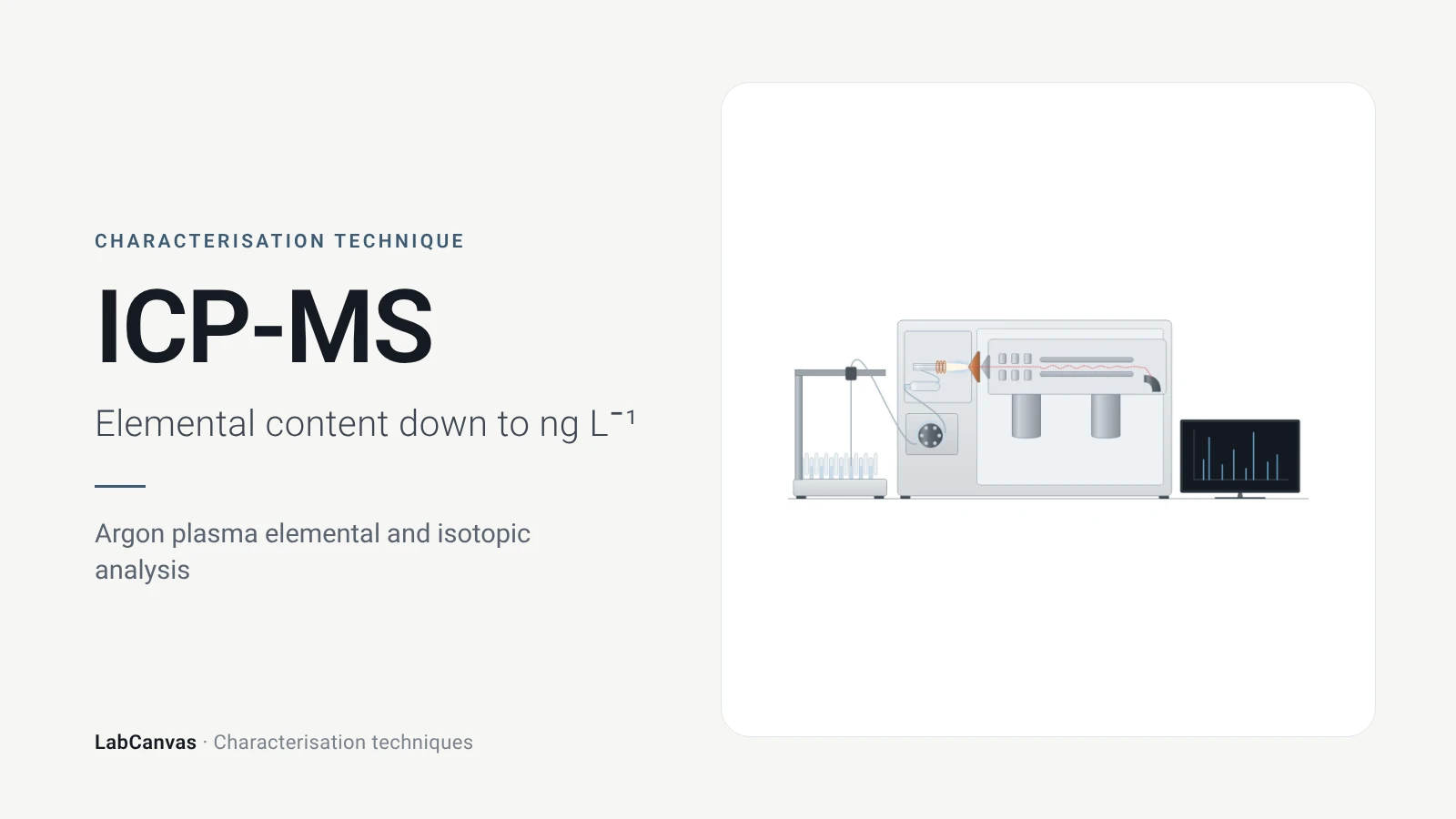
ICP-MS and ICP-OES
ICP-MS and ICP-OES explained: argon plasma, detection limits, acid digestion, interferences, single-particle ICP-MS and metal content of MOFs.
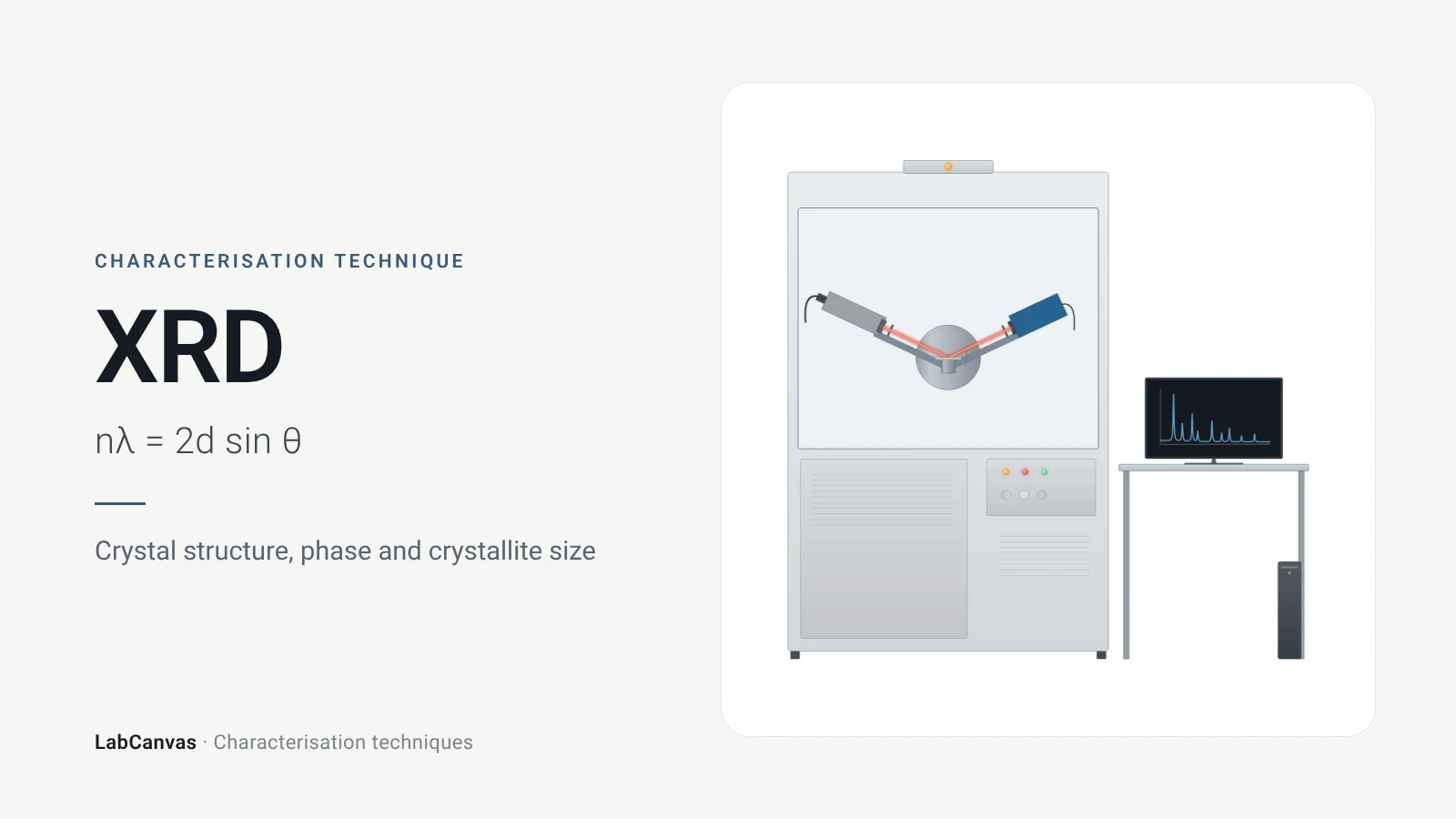
X-ray diffraction (XRD)
X-ray diffraction explained: Bragg’s law, how to read an XRD pattern, phase identification, Scherrer crystallite size, Rietveld refinement and common mistakes.
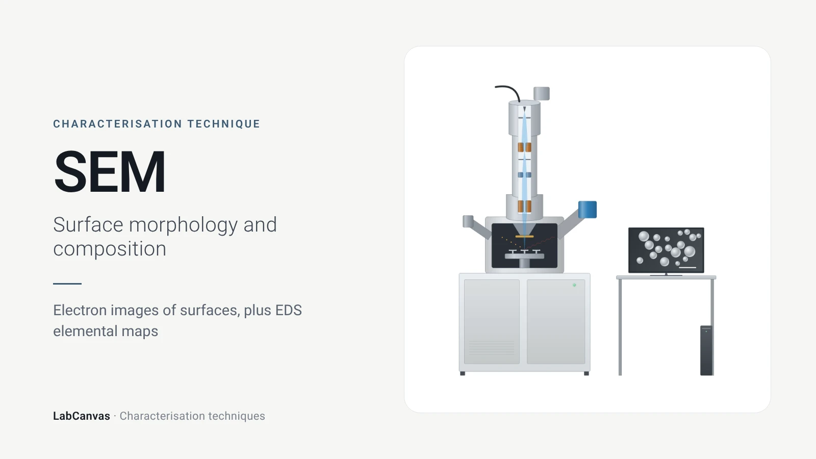
Scanning electron microscopy (SEM)
How SEM works: secondary vs backscattered electron images, EDS/EDX elemental analysis, resolution, sample coating, low-vacuum mode and common mistakes.
More on LabCanvas
- All characterisation techniques: XRD, XPS, BET, SEM, TEM, NMR, FTIR, Raman and more, explained with cited sources
- Graphical abstract sizes and templates: ACS, Wiley, Angewandte, RSC, Elsevier and Cell Press, with templates at the right size
- RHE potential calculator: Free tool
- Tafel slope calculator: Free tool
- Materials explained: MOFs, COFs, 2D materials, perovskites, batteries and zeolites, with cited facts
- Journal figure size guide: Column widths and resolutions for 38 journals
Frequently asked questions
What is electrochemical impedance spectroscopy used for?
EIS measures how an electrochemical cell responds to a small AC signal over many frequencies, separating electrolyte resistance, charge transfer, double-layer charging and diffusion (Lazanas & Prodromidis 2023). It is used in batteries, fuel cells, corrosion, electrocatalysis and biosensors.
How do you read a Nyquist plot?
Each point is one frequency, with −Z″ against Z′. For a Randles-type cell the high-frequency intercept is the solution resistance, the semicircle width is the charge-transfer resistance and a 45° line at low frequency is diffusion (Lazanas & Prodromidis 2023).
What is the Randles circuit?
The standard equivalent circuit for an electrode with a redox reaction: solution resistance in series with the double-layer capacitance, which is in parallel with the charge-transfer resistance and the Warburg diffusion impedance (Lazanas & Prodromidis 2023).
What is Warburg impedance?
The impedance of semi-infinite diffusion of redox species to the electrode, seen as a straight line at 45° at low frequencies in the Nyquist plot (Lazanas & Prodromidis 2023).
What does charge-transfer resistance tell you?
Rct reflects how fast electrons cross the electrode–electrolyte interface: a smaller Rct means faster charge transfer (Sondermann et al. 2025). For electrocatalysts it is compared at catalytic-turnover potentials (Sharma et al. 2026).
Nyquist vs Bode plot: what is the difference?
A Nyquist plot shows −Z″ against Z′ and hides frequency, while a Bode plot shows log|Z| and phase against log frequency, so you can see at which frequency each process occurs (Lazanas & Prodromidis 2023).
What amplitude and frequency range should I use for EIS?
Typically 5–10 mV under potentiostatic control (Lazanas & Prodromidis 2023), and a range from at least 10 kHz down to 1 Hz or lower so the charge-transfer arc is captured (Sharma et al. 2026).
What is a constant phase element?
A circuit element used instead of an ideal capacitor when arcs are depressed, often because of electrode roughness; its exponent n is 1 for a capacitor, 0.5 for Warburg diffusion and 0 for a resistor (Lazanas & Prodromidis 2023).
References
- A. Ch. Lazanas, M. I. Prodromidis. Electrochemical impedance spectroscopy—a tutorial. ACS Meas. Sci. Au 2023, 3, 162–193. doi:10.1021/acsmeasuresciau.2c00070
- M. Sharma, C. Prakash, V. K. Singh, A. Dixit. A tutorial on measurement of electrochemical water-splitting performance parameters: methods and best practices. ACS Meas. Sci. Au 2026, 6, 1445–1470. doi:10.1021/acsmeasuresciau.6c00147
- L. Sondermann, L. M. Voggenauer, A. Vollrath, T. Strothmann, C. Janiak. Comparison of in situ and postsynthetic formation of MOF-carbon composites as electrocatalysts for the alkaline oxygen evolution reaction (OER). Molecules 2025, 30, 208. doi:10.3390/molecules30020208
- T. H. Y. Beglau, L. Rademacher, R. Oestreich, C. Janiak. Synthesis of Ketjenblack decorated pillared Ni(Fe) metal-organic frameworks as precursor electrocatalysts for enhancing the oxygen evolution reaction. Molecules 2023, 28, 4464. doi:10.3390/molecules28114464
- T. Moehl, E. Service, W. Yang, S. D. Tilley. Electrochemical impedance spectroscopy of (photo)electrochemical systems: a practical guide. ACS Meas. Sci. Au 2026, 6, 1433–1444. doi:10.1021/acsmeasuresciau.6c00109
Draw Electrochemical impedance spectroscopy (EIS) figures for your paper
LabCanvas is a browser workspace for scientific figures: instruments with their beam and light paths, editable data plots, crystal structures, graphs and graphical abstracts at journal sizes.
Draw Electrochemical impedance spectroscopy (EIS) in LabCanvas