Dynamic light scattering (DLS) and zeta potential: how they work and how to read size, PDI and ζ
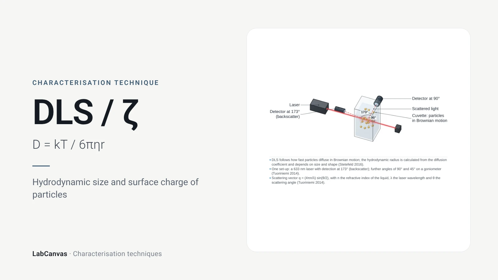
Dynamic light scattering (DLS) shines a laser into a dilute dispersion and records how fast the scattered intensity fluctuates as particles move by Brownian motion; small particles move quickly and large ones slowly (Rodriguez-Loya et al. 2023). The decay of the intensity autocorrelation gives a diffusion coefficient, which the Stokes–Einstein equation turns into a hydrodynamic diameter (Wishard & Gibb 2019), and a cumulants fit gives the polydispersity index, PDI (Danaei et al. 2018). Zeta potential is measured in the same instruments by electrophoretic light scattering: the particle velocity in an electric field gives the electrophoretic mobility and, through Henry's equation, the potential at the slipping plane, with values beyond about ±30 mV usually read as a stable dispersion (Rodriguez-Loya et al. 2023).
Contents
DLS and zeta potential at a glance
| Probe | A laser beam through a dilute liquid dispersion (Wishard & Gibb 2019) |
|---|---|
| Signal measured (DLS) | Time fluctuations of scattered intensity, analysed as an autocorrelation function (Wishard & Gibb 2019) |
| Key equation | Stokes–Einstein: D = k_BT / (6πηr_H) links the diffusion coefficient to the hydrodynamic radius (Wishard & Gibb 2019) |
| Main information | Hydrodynamic diameter and its distribution, PDI, aggregation over time; zeta potential from electrophoretic mobility (Rodriguez-Loya et al. 2023; Danaei et al. 2018) |
| Size range | From about 1 nm upwards for DLS (Danaei et al. 2018); a few nanometres to several micrometres (Rodriguez-Loya et al. 2023) |
| Intensity weighting | Scattered intensity scales with d⁶, so a 10 nm particle scatters 10⁶ times more than a 1 nm one (Wishard & Gibb 2019) |
| PDI | From the cumulants fit; < 0.05 only for highly monodisperse standards, > 0.7 too broad for DLS; ≤ 0.3 accepted for lipid carriers and ≤ 0.2 for polymer nanoparticles (Danaei et al. 2018) |
| Zeta potential | Potential at the slipping plane from electrophoretic mobility via Henry's equation, f(κa) = 1.5 (Smoluchowski) or 1.0 (Hückel) (Rodriguez-Loya et al. 2023) |
| Stability rule of thumb | Beyond about ±30 mV generally stable; closer to zero less stable; always report the pH (Rodriguez-Loya et al. 2023) |
| Standards | Size and PDI calculations defined in ISO 13321 and ISO 22412 (Danaei et al. 2018) |
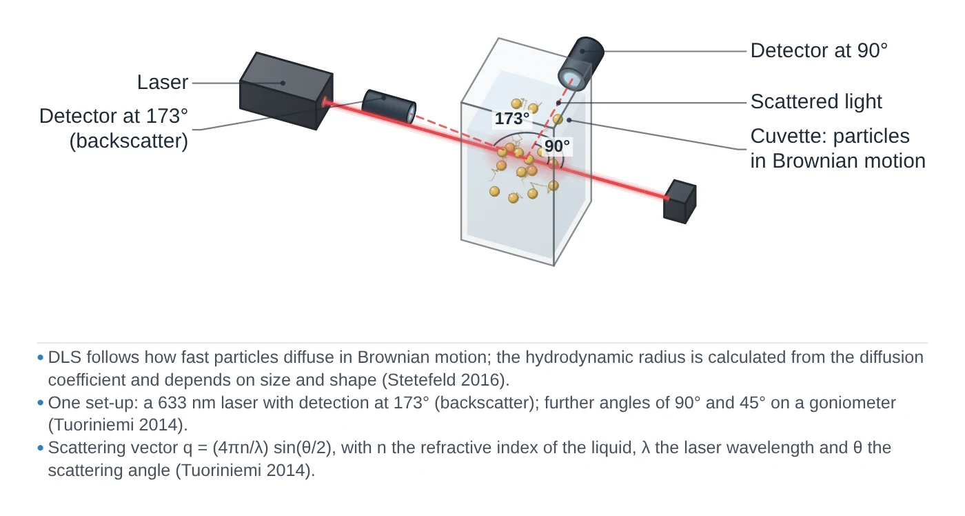
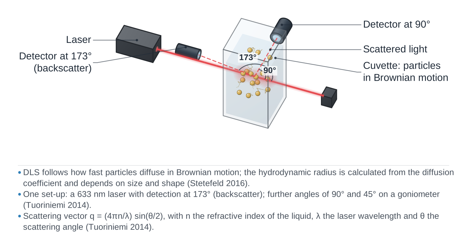
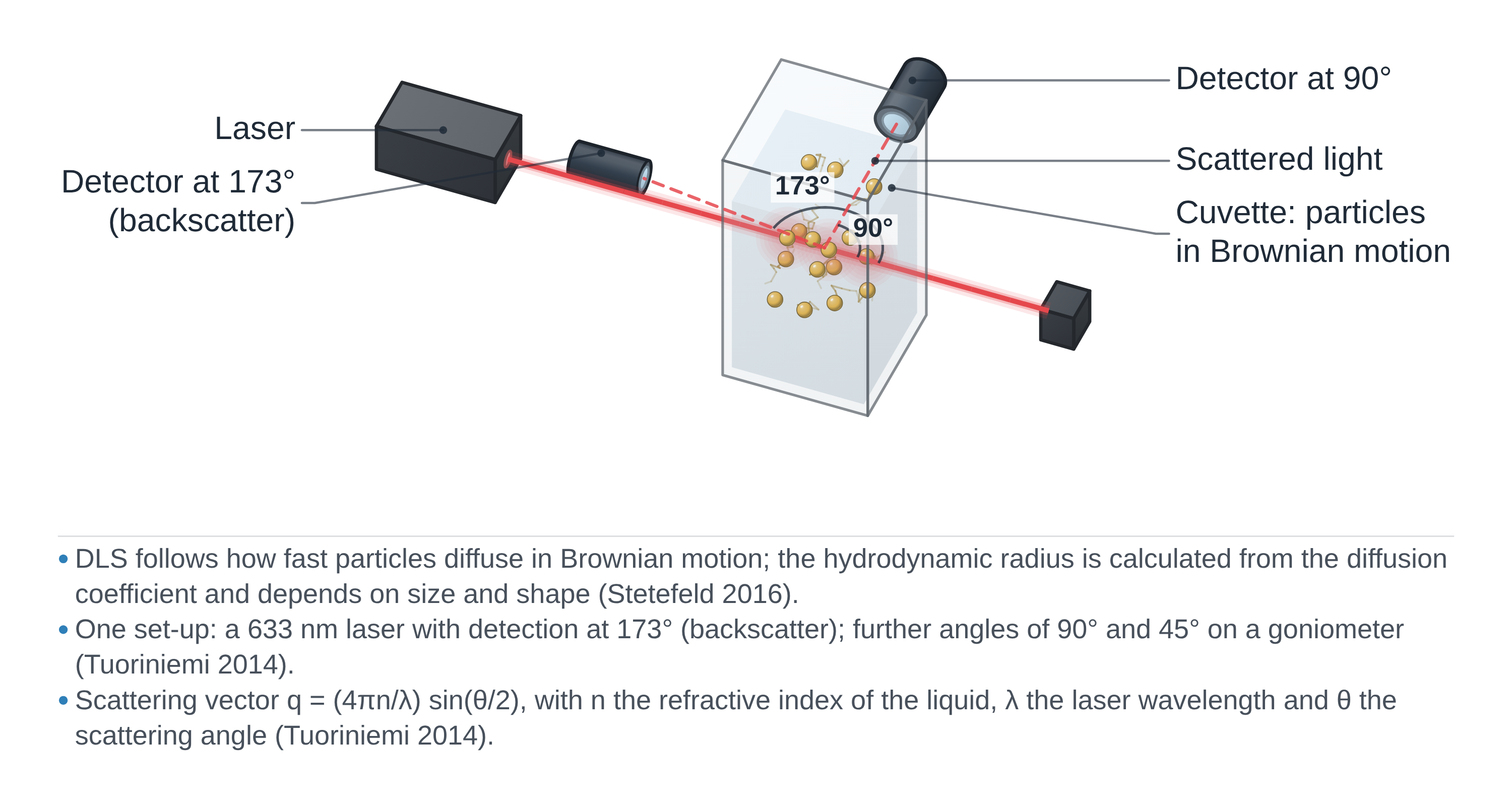
DLS and zeta potential instrument drawing (high-resolution SVG)
DLS and zeta potential data: an example plot to edit
How DLS and zeta potential work
Brownian motion and scattered light. Particles in a liquid move randomly because of collisions with solvent molecules; small particles move fast and large ones slowly (Rodriguez-Loya et al. 2023). When a laser lights the sample, light scattered by all the particles interferes, and as they move the total scattered intensity fluctuates. DLS records these fluctuations in time, whereas static light scattering records only the time-averaged intensity (Wishard & Gibb 2019).
From fluctuations to size. A correlator compares the intensity at time t with the intensity a delay τ later. For short delays the signal is well correlated; as τ grows the correlation decays, usually exponentially, as g₂(τ) = 1 + β·exp(−2Dq²τ), where D is the translational diffusion coefficient and q the scattering vector (Wishard & Gibb 2019). In a typical measurement the correlation falls away within about 1–10 ms (Rodriguez-Loya et al. 2023). The diffusion coefficient is then converted to a hydrodynamic radius with the Stokes–Einstein equation, D = k_BT / (6πηr_H), where η is the viscosity of the liquid and T the temperature (Wishard & Gibb 2019). The result is a sphere-equivalent hydrodynamic size: for non-spherical particles the measured diffusion mixes translation and rotation (Wishard & Gibb 2019).
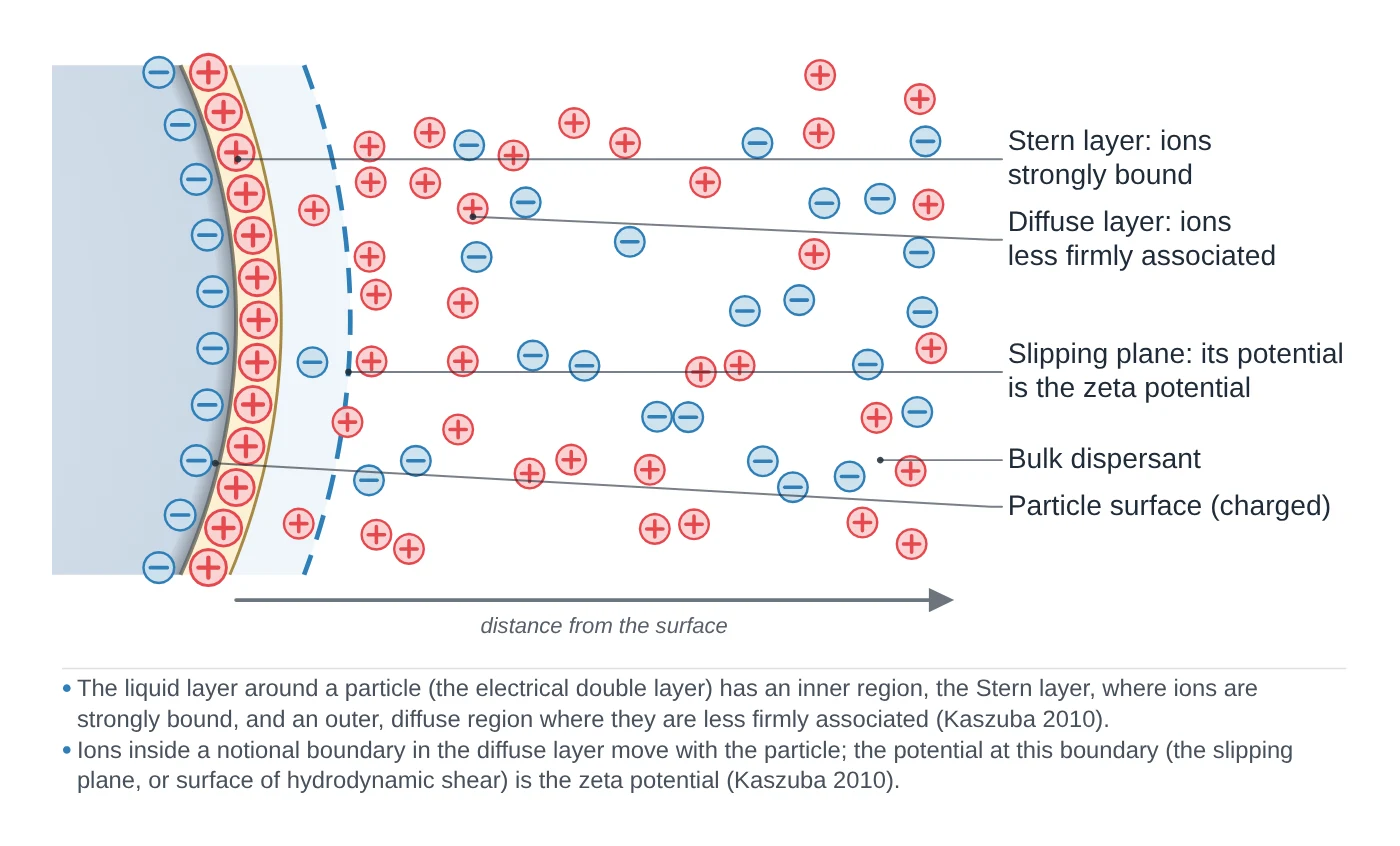
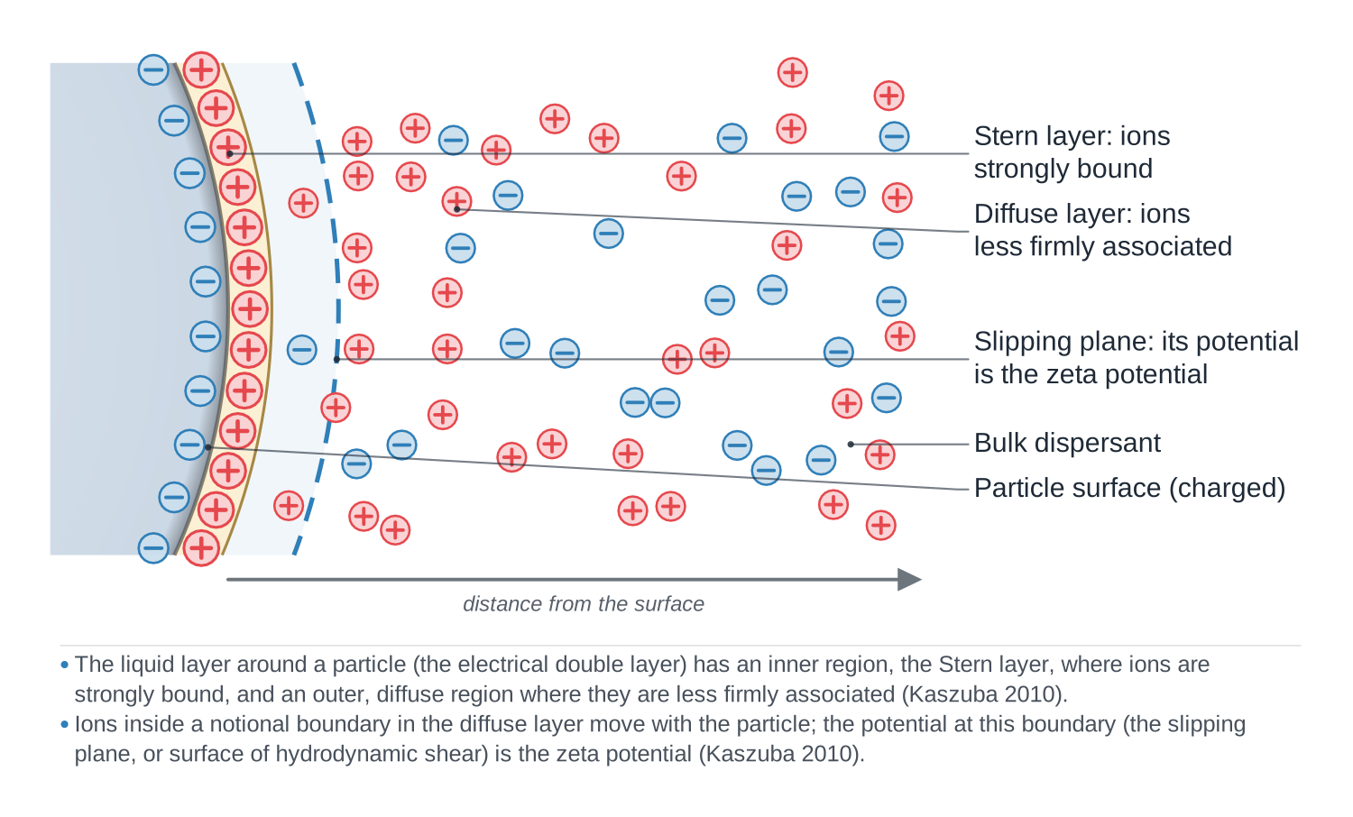
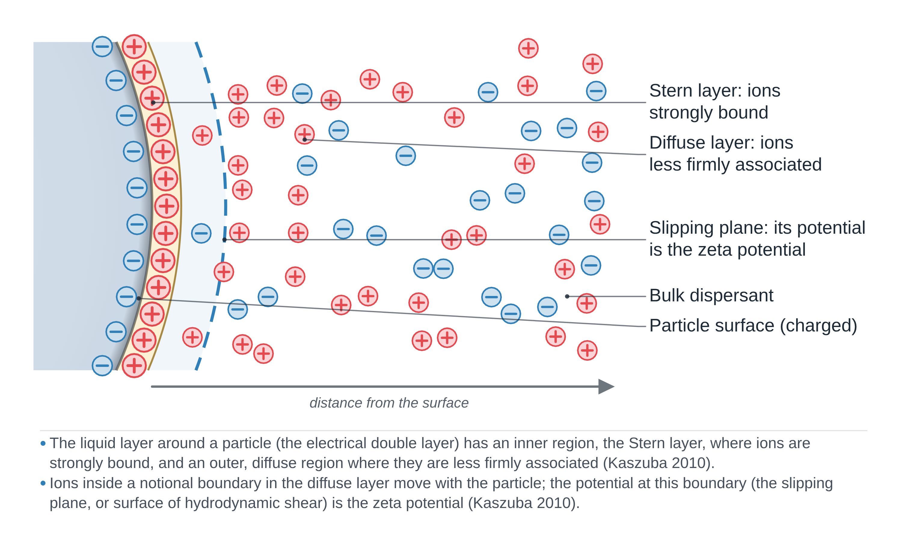
Zeta potential. In electrophoretic light scattering, the instrument applies an electric field and measures how fast the particles move, using laser Doppler velocimetry: the scattered light is Doppler-shifted by the moving particles (Rodriguez-Loya et al. 2023). The velocity per unit field is the electrophoretic mobility U_E, and Henry's equation, U_E = 2εζf(κa)/3η, converts it to the zeta potential ζ, the electrical potential at the slipping plane between the particle and the bulk liquid. For particles that are large compared with the double layer in aqueous salt solutions f(κa) = 1.5 (the Smoluchowski limit); for small particles in low-salt or low-dielectric media f(κa) = 1.0 (the Hückel limit) (Rodriguez-Loya et al. 2023). These two measurements belong with the other characterisation techniques for anything dispersed in a liquid.
What the data looks like and how to read it
Start with the correlation function. It is the raw data of DLS. A clean curve starts high and decays smoothly to a flat baseline; a noisy, poorly correlated curve, caused by weak scattering, dust, precipitation or sedimentation, gives unreliable sizes whatever the software reports (Wishard & Gibb 2019).
Mean size and PDI. The cumulants method fits the correlation function of a single population and gives a mean size and the polydispersity index (Wishard & Gibb 2019; Danaei et al. 2018). PDI runs from 0 for a perfectly uniform sample to 1 for a very broad one; below 0.05 is seen only with highly monodisperse standards, and above 0.7 the distribution is probably too broad for DLS. In practice 0.2 or less is accepted for polymer nanoparticles and 0.3 or less for liposomes and other lipid carriers (Danaei et al. 2018).
Intensity, volume and number distributions. For several populations, software fits the decay with an NNLS-type algorithm and reports a size distribution (Wishard & Gibb 2019). The intensity distribution is the primary result; volume and number distributions are calculated from it with Mie theory (Rodriguez-Loya et al. 2023). Because scattered intensity scales with the sixth power of diameter, a 1:1 mixture by number of 1 nm and 10 nm particles shows up as 1:10⁶ by intensity and about 1:1000 by volume (Wishard & Gibb 2019). Likewise, equal numbers of 50 nm and 100 nm particles give an intensity ratio of 1:64 (calculated from I ∝ d⁶). A small peak of large particles in the intensity plot can therefore be only a tiny number of aggregates.
Zeta potential. The result is a value in millivolts with its sign, usually shown as a distribution. A value beyond about ±30 mV is generally taken as the line between stable and unstable dispersions, values near zero as unstable; some authors ask for ±40 to ±60 mV for good stability (Rodriguez-Loya et al. 2023). Always quote the pH and the medium alongside it (Rodriguez-Loya et al. 2023).
Sample preparation
- Keep it dust-free. Because of the d⁶ scaling, one dust particle can swamp the signal of nanometre particles; use clean, capped cuvettes and wipe the outside (Wishard & Gibb 2019).
- Centrifuge or filter. Centrifuging for about 10 min at 10,000 rpm or filtering removes stray particles; measure an unfiltered reference too, so you know the filter did not remove your own aggregates (Wishard & Gibb 2019).
- Dilute. The sample must be dilute enough to avoid multiple scattering (Rodriguez-Loya et al. 2023); concentration effects are also one cause of DLS–TEM disagreement (Filippov et al. 2023).
- Enter the right solvent data and wait for temperature. The viscosity and refractive index of the solvent at the measurement temperature are needed, and each degree away from thermal equilibrium adds about 2% error to the size (Wishard & Gibb 2019).
- Choose the angle. Back-scatter at about 173° suits large particles; about 90° suits small ones, where forward scatter from large species would otherwise dominate (Wishard & Gibb 2019).
- Add background salt for charged particles. Unscreened polyelectrolytes diffuse anomalously fast and look too small; salt or buffer removes the effect (Wishard & Gibb 2019). For zeta potential, control pH and ionic strength, which set the double-layer thickness (Rodriguez-Loya et al. 2023).
What DLS and zeta potential tell you about materials
Colloidal stability and aggregation. DLS follows particle size over time, so it shows aggregation as it happens, and zeta potential gives the electrostatic part of the stability (Rodriguez-Loya et al. 2023). In DLVO theory, the stability of a dispersion is the balance of van der Waals attraction and electric double-layer repulsion; adding salt compresses the double layer and screens the repulsion, which is why dispersions that are stable at low salt aggregate at high salt (Rodriguez-Loya et al. 2023).
Isoelectric point. Measuring zeta potential across a pH range finds the isoelectric point, where the dispersion is least stable (Rodriguez-Loya et al. 2023). The same size and zeta measurements apply to dispersions of MOF nanoparticles such as ZIF-8 or UiO-66 and to sheets such as graphene oxide, whose non-spherical shape limits what a sphere-equivalent size means (Wishard & Gibb 2019).
Nanocarriers and quality control. Size and PDI are critical quality attributes of lipid nanoparticles and liposomes, measured by DLS against ISO 13321 and ISO 22412 (Danaei et al. 2018).
Size in solution, not dry size. DLS gives an ensemble hydrodynamic size of particles in their liquid; it complements TEM and SEM, which image dry particles one by one (Danaei et al. 2018). For crystallite size from diffraction, see XRD; for gold nanoparticles, the plasmon band in UV–vis gives another size estimate.
Common mistakes and limits
- Reporting the number distribution as "the size". The intensity distribution is what DLS measures; volume and number distributions are conversions from it through Mie theory (Rodriguez-Loya et al. 2023; Wishard & Gibb 2019). Report the intensity result and say which weighting you show.
- Expecting DLS to match TEM. Many papers report DLS and TEM sizes that differ by 200–300%; concentration and angle effects are common causes, and correct procedures bring the two much closer (Filippov et al. 2023). DLS also counts an aggregate of several particles as one particle (Danaei et al. 2018).
- Applying it to non-spheres without care. For rods and sheets the measured diffusion mixes translation and rotation, so the sphere-equivalent size is only indicative (Wishard & Gibb 2019); DLS gives no shape information (Danaei et al. 2018).
- Measuring broad or concentrated samples. A PDI above about 0.7 means the sample is probably not suitable for DLS (Danaei et al. 2018); high concentration, high viscosity and turbidity reduce reliability (Rodriguez-Loya et al. 2023).
- Quoting ζ without conditions. Zeta potential depends on pH, conductivity, temperature and the ions present (Rodriguez-Loya et al. 2023); a value without pH and medium cannot be compared.
- Forgetting that ELS can change the sample. The applied current can damage sensitive samples, so measure size before zeta potential (Wishard & Gibb 2019).
How to draw the DLS setup and data in LabCanvas
In the LabCanvas figure editor, the Library has a DLS / zeta potential analyser as an editable object, including a cutaway of the laser path through the cuvette to the detector at the back-scatter and side-scatter angles and the electrodes of the zeta cell, plus an editable data plot for correlation functions, intensity, volume and number distributions and zeta potential curves. You can label the peaks with their hydrodynamic diameters and the PDI, mark the ±30 mV stability band, and export the figure for a methods section or a graphical abstract.
DLS compared with other particle sizing methods
| Technique | What it measures | Sample | Range / output |
|---|---|---|---|
| DLS | Intensity fluctuations from Brownian motion → diffusion coefficient → hydrodynamic size | Dilute liquid dispersion | Down to ~1 nm; ensemble mean size and PDI, no shape (Danaei et al. 2018) |
| Nanoparticle tracking analysis (NTA) | Brownian motion of individual particles tracked on video, sized by Stokes–Einstein | Liquid dispersion | 30–1000 nm; size distribution and concentration (Danaei et al. 2018) |
| Electron microscopy (TEM, SEM) | Images of individual dried particles | Particles on a grid or substrate | Shape and size of a limited number of particles (Danaei et al. 2018) |
| SAXS | X-ray scattering at small angles from density differences | Liquid or solid | Size distribution and shape of monodisperse samples (Danaei et al. 2018) |
Related techniques
UV–vis spectroscopy
UV–vis spectroscopy explained: absorbance and the Beer–Lambert law, band gap from a Tauc plot, diffuse reflectance for powders and gold plasmon bands.
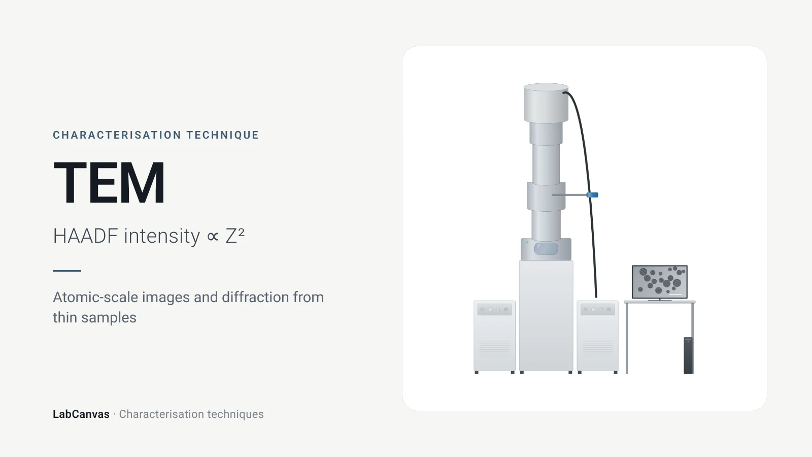
Transmission electron microscopy (TEM)
How TEM works: bright field, HRTEM lattice images, SAED diffraction, STEM-HAADF Z-contrast, EDS/EELS, sample thickness and beam damage of MOFs.
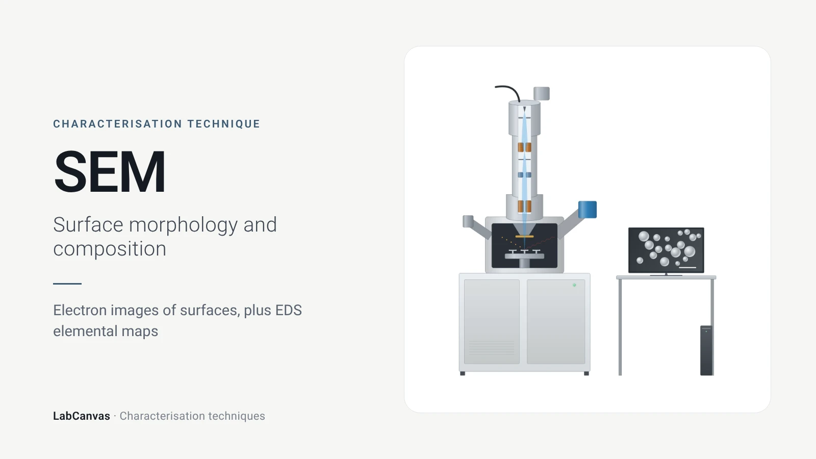
Scanning electron microscopy (SEM)
How SEM works: secondary vs backscattered electron images, EDS/EDX elemental analysis, resolution, sample coating, low-vacuum mode and common mistakes.
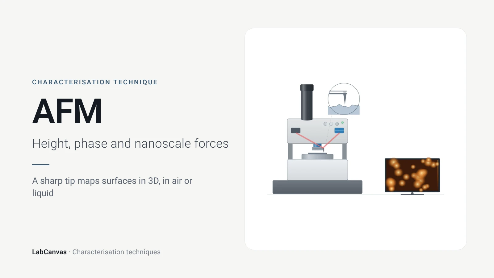
Atomic force microscopy (AFM)
How AFM works: tip, cantilever and laser deflection, contact vs tapping mode, measuring 2D flake thickness from height profiles, and common AFM artefacts.
More on LabCanvas
- All characterisation techniques: XRD, XPS, BET, SEM, TEM, NMR, FTIR, Raman and more, explained with cited sources
- Graphical abstract sizes and templates: ACS, Wiley, Angewandte, RSC, Elsevier and Cell Press, with templates at the right size
- Materials explained: MOFs, COFs, 2D materials, perovskites, batteries and zeolites, with cited facts
- Journal figure size guide: Column widths and resolutions for 38 journals
Frequently asked questions
What does DLS measure?
DLS measures how fast the light scattered by particles in a liquid fluctuates as they move by Brownian motion. The decay of the intensity autocorrelation gives a diffusion coefficient, which the Stokes–Einstein equation converts to a hydrodynamic diameter (Wishard & Gibb 2019).
What is the hydrodynamic diameter?
It is the diameter calculated from the particle's measured diffusion coefficient with the Stokes–Einstein equation, D = k_BT/(6πηr_H), treating the particle as a sphere; for non-spherical particles the diffusion also contains rotation, so it is a sphere-equivalent size (Wishard & Gibb 2019).
What is a good PDI value in DLS?
PDI runs from 0 (uniform) to 1 (very broad). Values below 0.05 are seen only for highly monodisperse standards, 0.2 or less is accepted for polymer nanoparticles and 0.3 or less for lipid carriers, and above 0.7 the sample is probably unsuitable for DLS (Danaei et al. 2018).
Intensity vs number distribution in DLS: which should I report?
The intensity distribution is the primary DLS result; volume and number distributions are derived from it (Rodriguez-Loya et al. 2023). Because intensity scales with d⁶, a 1:1 number mixture of 1 nm and 10 nm particles appears as 1:10⁶ by intensity (Wishard & Gibb 2019). Report the intensity result and state which weighting any other plot uses.
Why is my DLS size larger than the TEM size?
DLS measures particles in liquid as an intensity-weighted ensemble that counts aggregates as single particles (Danaei et al. 2018), and scattered intensity scales with d⁶, so large particles dominate (Wishard & Gibb 2019). Differences of 200–300% are common, though careful control of concentration and angle brings the two much closer (Filippov et al. 2023).
What is zeta potential?
Zeta potential is the electrical potential at the slipping plane around a particle in a liquid. It is calculated from the electrophoretic mobility measured by laser Doppler velocimetry, using Henry's equation with f(κa) = 1.5 (Smoluchowski) or 1.0 (Hückel) (Rodriguez-Loya et al. 2023).
What zeta potential value means a stable dispersion?
About ±30 mV is generally accepted as the dividing line: beyond it dispersions are usually stable, closer to zero they tend to aggregate; some authors ask for ±40 to ±60 mV for good stability (Rodriguez-Loya et al. 2023).
DLS vs NTA: what is the difference?
Both use Brownian motion and the Stokes–Einstein equation, but DLS analyses the fluctuating intensity of the whole ensemble, down to about 1 nm, while nanoparticle tracking analysis follows individual particles on video over about 30–1000 nm and also gives concentration (Danaei et al. 2018).
References
- A. Wishard, B. C. Gibb. Dynamic light scattering – an all-purpose guide for the supramolecular chemist. Supramol. Chem. 2019, 31, 608–615. doi:10.1080/10610278.2019.1629438
- J. Rodriguez-Loya, M. Lerma, J. L. Gardea-Torresdey. Dynamic light scattering and its application to control nanoparticle aggregation in colloidal systems: a review. Micromachines 2023, 15, 24. doi:10.3390/mi15010024
- M. Danaei et al.. Impact of particle size and polydispersity index on the clinical applications of lipidic nanocarrier systems. Pharmaceutics 2018, 10, 57. doi:10.3390/pharmaceutics10020057
- S. K. Filippov et al.. Dynamic light scattering and transmission electron microscopy in drug delivery: a roadmap for correct characterization of nanoparticles and interpretation of results. Mater. Horiz. 2023, 10, 5354–5370. doi:10.1039/d3mh00717k
Draw DLS and zeta potential figures for your paper
LabCanvas is a browser workspace for scientific figures: instruments with their beam and light paths, editable data plots, crystal structures, graphs and graphical abstracts at journal sizes.
Draw DLS and zeta potential in LabCanvas