UV–vis spectroscopy: how it works, the Beer–Lambert law, band gaps from Tauc plots and plasmon bands
UV–vis spectroscopy measures how much ultraviolet and visible light a sample absorbs at each wavelength, usually reported as absorbance, the negative decadic logarithm of the transmittance (Mayerhöfer et al. 2019). By the Beer–Lambert law absorbance is proportional to concentration and path length, A = εcl, which makes UV–vis the everyday way to measure concentration (Mayerhöfer et al. 2019). For semiconductors the absorption edge gives the optical band gap through a Tauc plot, with diffuse reflectance used for powders (Escobedo-Morales et al. 2019), and for gold nanoparticles the plasmon band reports size, concentration and aggregation (Haiss et al. 2007; Wang et al. 2026).
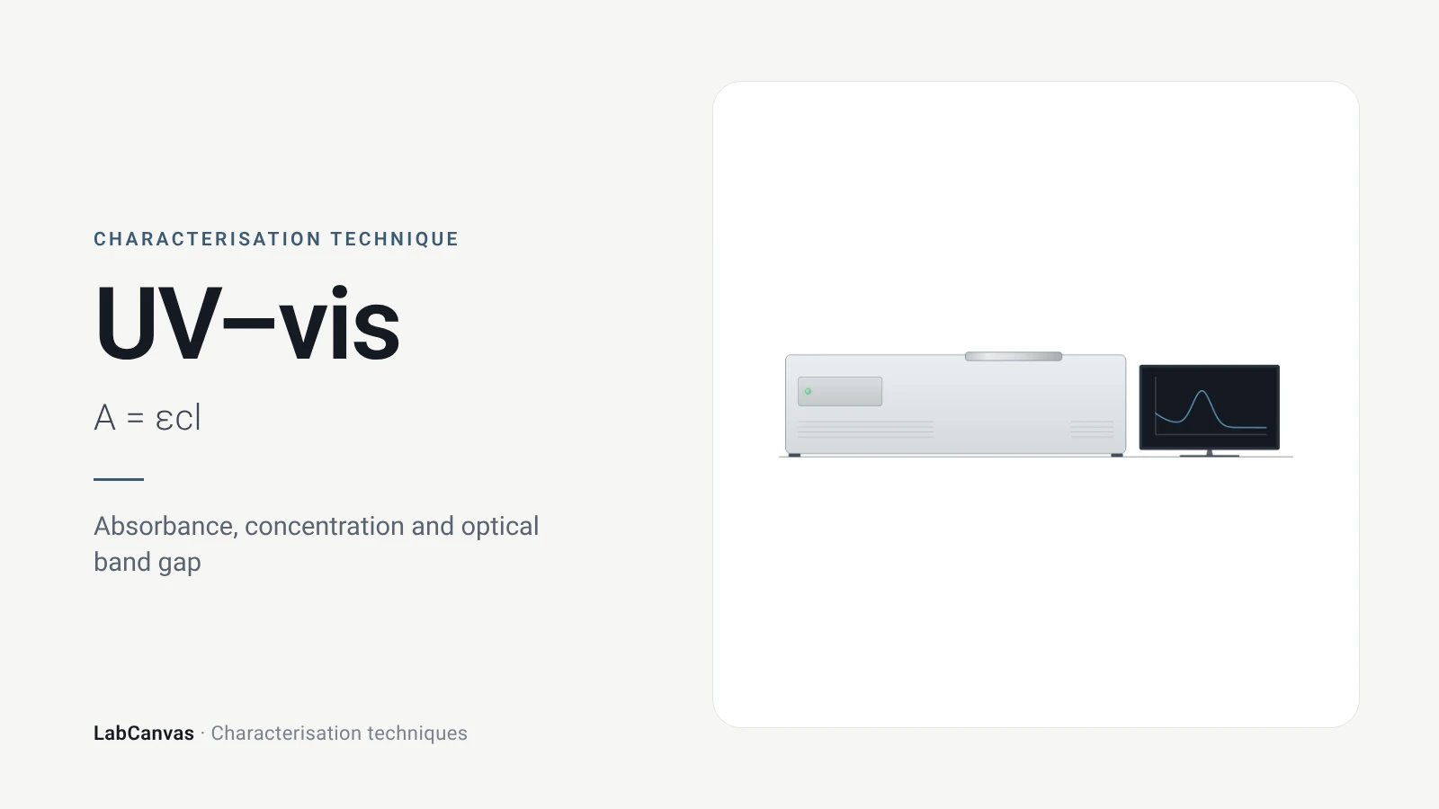
Contents
UV–vis spectroscopy at a glance
| Probe | Ultraviolet and visible light, scanned in wavelength (Mayerhöfer et al. 2019) |
|---|---|
| Signal measured | Transmittance, converted to absorbance A = −log₁₀T, ratioed to the pure solvent in practice (Mayerhöfer et al. 2019); for powders, diffuse reflectance against a PTFE or BaSO₄ standard (Escobedo-Morales et al. 2019) |
| Key law | Beer–Lambert: A = εcd, with ε the molar attenuation coefficient, c the concentration and d the path length (Mayerhöfer et al. 2019) |
| Main information | Concentration (Mayerhöfer et al. 2019); optical band gap from a Tauc plot (Escobedo-Morales et al. 2019); plasmon band position and strength of metal nanoparticles (Haiss et al. 2007) |
| Band gap relation | (αhν)^(1/n) = C(hν − Eg); n = 1/2 direct allowed, 3/2 direct forbidden, 2 indirect allowed, 3 indirect forbidden (Escobedo-Morales et al. 2019) |
| Powders | Use diffuse reflectance and the Kubelka–Munk function F(R∞) in place of α; sample layer thicker than about 2 mm (Escobedo-Morales et al. 2019) |
| Example band gaps | ZnO 3.25 eV by DRS and Tauc; CdO about 2.2 eV; Al₂O₃ about 5 eV (Escobedo-Morales et al. 2019) |
| Gold nanoparticles | Plasmon band near 520 nm when dispersed; red-shifts and broadens on aggregation (Wang et al. 2026); size and concentration readable for 5–100 nm particles (Haiss et al. 2007) |
| Linearity limits | Monochromatic light, no chemical interactions, adequate spectral resolution and a linear detector are assumed (Mayerhöfer et al. 2019; Li et al. 2022) |
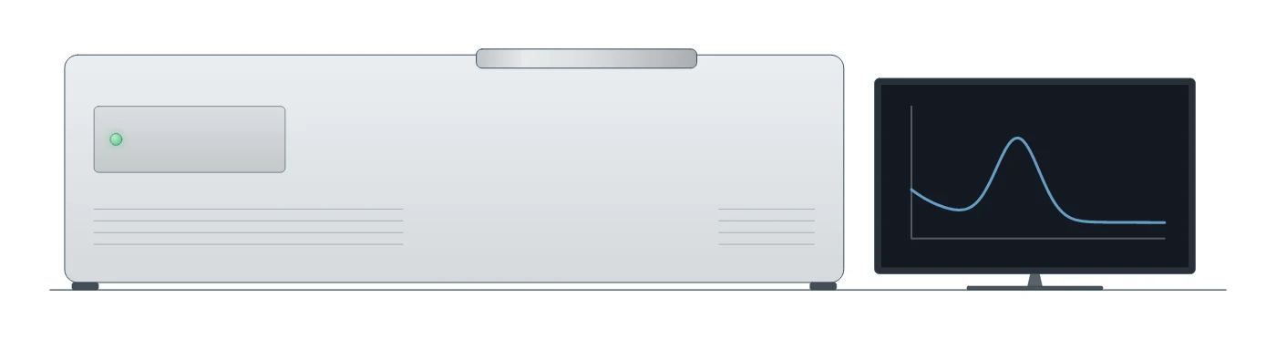
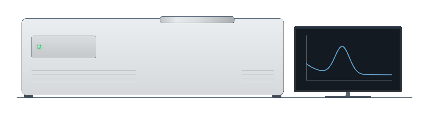
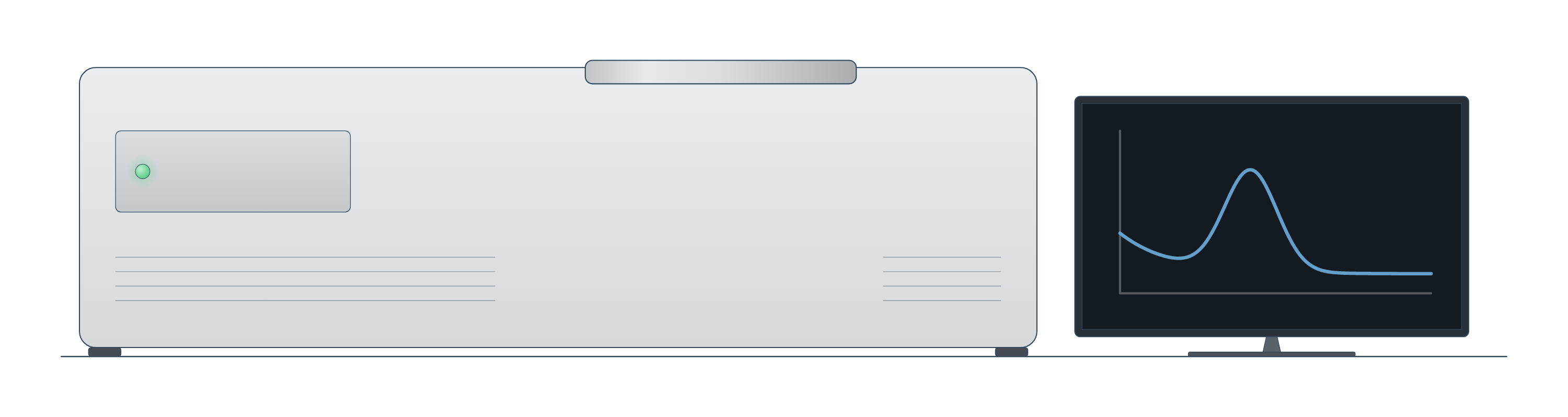
UV–vis spectroscopy instrument drawing (high-resolution SVG)
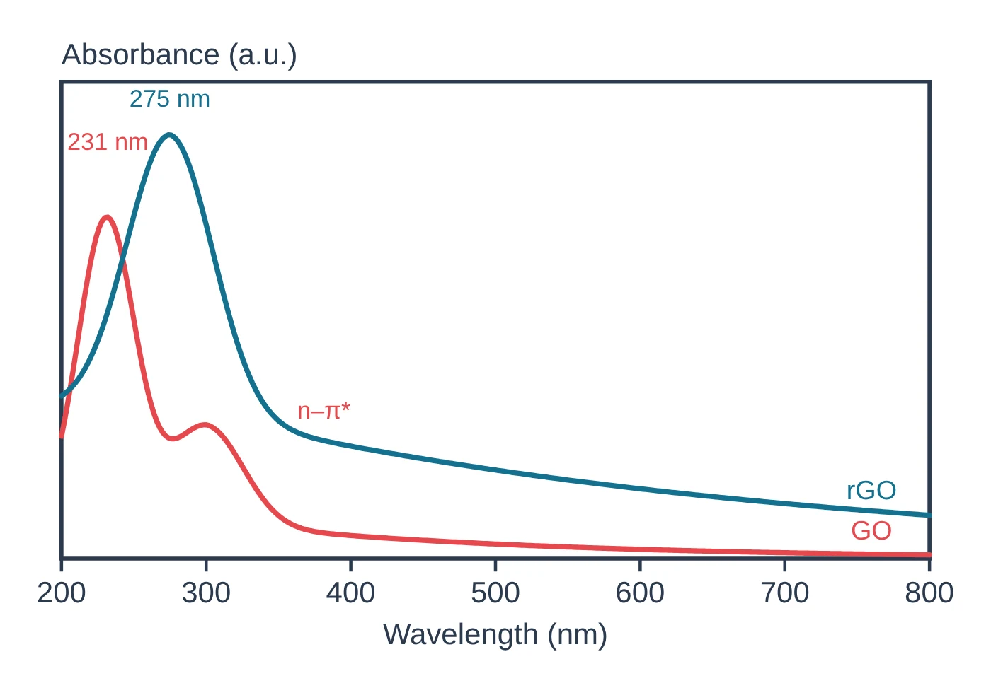
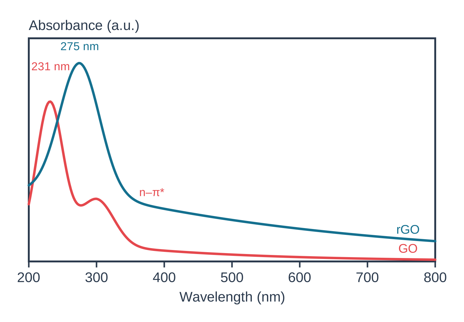
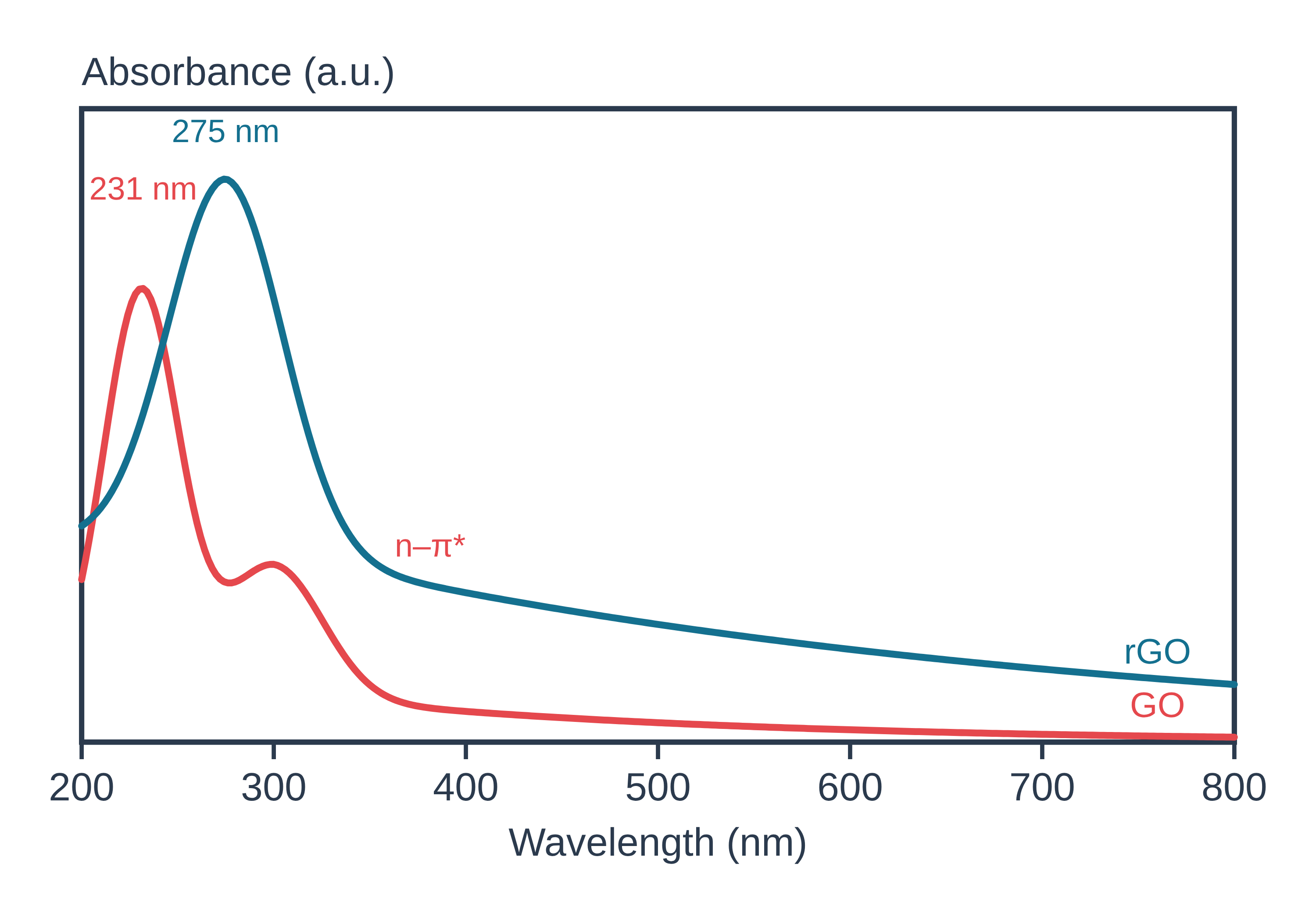
UV–vis spectroscopy data: an example plot to edit
How UV–vis works
A spectrometer passes ultraviolet and visible light through a sample, usually a solution in a cuvette, and compares the light that comes out with the light that went in. The ratio is the transmittance T, and the quantity plotted is the absorbance, A = −log₁₀T; in routine work the transmittance of the solution is ratioed to that of the pure solvent, which removes the baseline (Mayerhöfer et al. 2019).
The Beer–Lambert law links absorbance to the amount of absorber: A = εcl, where ε is the molar attenuation coefficient, c the concentration and l the path length. Beer showed in 1852 that the transmittance stays the same when the product of cell thickness and concentration stays the same (Mayerhöfer et al. 2019). The law assumes monochromatic light and absorbers that do not interact; finite spectral resolution, detector nonlinearity, chemical interactions, scattering and plasmonic field enhancement all make it fail (Mayerhöfer et al. 2019).
For a semiconductor, light is absorbed once the photon energy reaches the band gap, so the spectrum has an absorption edge. ZnO, for instance, absorbs below about 380 nm, which corresponds to its gap of about 3.3 eV (Escobedo-Morales et al. 2019). UV–vis sits with the other characterisation techniques as the quickest optical measurement.
What the data looks like and how to read it
Solutions. A UV–vis spectrum plots absorbance against wavelength. Read the wavelength of maximum absorbance and its height; at a fixed wavelength, absorbance rises linearly with concentration, so a calibration line of A against c gives unknown concentrations (Mayerhöfer et al. 2019).
Band gap from a Tauc plot. The Tauc method relates the absorption coefficient α to the photon energy hν:
(αhν)^(1/n) = C(hν − Eg)
where n = 1/2 for a direct allowed transition, 3/2 for direct forbidden, 2 for indirect allowed and 3 for indirect forbidden (Escobedo-Morales et al. 2019). Plot (αhν)^(1/n) against hν, fit a straight line to the steep part of the absorption edge (the Tauc segment) and read Eg where that line meets the energy axis (Escobedo-Morales et al. 2019). Convert wavelength to energy with E (eV) ≈ 1240 / λ (nm) (calculated from E = hc/λ; it reproduces ZnO's 3.3 eV ≈ 375 nm in Escobedo-Morales et al. 2019).
You can do this without a spreadsheet: the free LabCanvas Tauc plot band gap calculator takes absorbance against wavelength or photon energy (or Kubelka–Munk F(R) values for powders, pasted in place of absorbance), lets you choose a direct or indirect allowed transition, subtracts a flat baseline below the gap, suggests the linear region of the edge and gives Eg from the intercept, with the plot as PNG or SVG and the data as CSV.
Powders: diffuse reflectance. Because the Tauc method uses α, it needs negligible scattering, and powders scatter strongly. For them, measure diffuse reflectance against a white standard (PTFE or BaSO₄), take R∞ as the ratio of sample to standard reflectance, and use the Kubelka–Munk function F(R∞) = (1 − R∞)² / 2R∞, which is proportional to the ratio of the absorption and scattering coefficients, in place of α (Escobedo-Morales et al. 2019).
Gold nanoparticles. Dispersed gold nanoparticles show a localised surface plasmon band near 520 nm, the source of their wine-red colour; when they aggregate, the band red-shifts and broadens and a new band can appear further to the red, turning the dispersion purple or blue (Wang et al. 2026). Because the band depends on particle size, the spectrum alone can give the size and concentration of spherical gold particles from 5 to 100 nm (Haiss et al. 2007).
Sample preparation
- Solutions. Use a matched cuvette of pure solvent as the reference, so the reported absorbance is ratioed to the solvent (Mayerhöfer et al. 2019).
- Stay in the linear range. Deviations from Beer–Lambert grow with higher concentration × path length and with poorer spectral resolution and lower light intensity (Li et al. 2022); dilute until A is proportional to c.
- Powders. Fill a holder deep enough (more than about 2 mm) that the holder does not contribute, and measure against a PTFE or BaSO₄ reflectance standard (Escobedo-Morales et al. 2019).
- Nanoparticle dispersions. Measure them well dispersed; aggregation changes the plasmon band itself (Wang et al. 2026). Check the hydrodynamic size and stability with DLS and zeta potential.
What UV–vis tells you about materials
Band gaps of semiconductors and photocatalysts. Optical spectroscopy with the Tauc method is by far the most widely used way to determine the band gap of a material (Escobedo-Morales et al. 2019). The same procedure applies to any semiconductor film or powder, for example the halide perovskites such as MAPbI₃ and CsPbBr₃ or layered MoS₂; automated algorithms now fit Tauc plots, including the choice between direct and indirect gaps, across many spectra at once (Suram et al. 2016).
Mixtures and composites. In a powder with more than one absorbing phase, the edge of the narrower-gap phase raises the background under the wider-gap edge. Intersecting the Tauc line with the energy axis then underestimates the wider gap: ZnO mixed with CoO gave 3.15 eV instead of 3.25 eV, while intersecting with a baseline segment recovered 3.24 eV (Escobedo-Morales et al. 2019).
Nanoparticles. For gold, the plasmon band gives particle size and concentration (Haiss et al. 2007) and shows aggregation as a red shift and broadening, the basis of colorimetric sensors (Wang et al. 2026).
Concentration. In solution chemistry, UV–vis with a Beer–Lambert calibration is the routine way to measure how much of a species is present (Mayerhöfer et al. 2019).
Common mistakes and limits
- Using the wrong exponent. The Tauc exponent must match the transition (n = 1/2 direct allowed, 2 indirect allowed); the wrong one gives the wrong gap (Escobedo-Morales et al. 2019).
- Ignoring the baseline. Absorption below the gap (defects, other phases, scattering) bends the Tauc plot; extrapolating to the axis can give large errors, and removing the baseline first gives a converging value, as for cubic BAs at 1.835 eV (Zhong et al. 2023). In mixtures, intersect with a baseline segment rather than the axis (Escobedo-Morales et al. 2019).
- Measuring powders in transmission. Scattering makes the absorbance of a powder meaningless for a Tauc plot; use diffuse reflectance with Kubelka–Munk (Escobedo-Morales et al. 2019).
- Trusting Beer–Lambert at high absorbance. Linearity fails at high concentration, poor resolution and low light levels (Li et al. 2022) and when absorbers interact (Mayerhöfer et al. 2019); integrated band area stays linear longer than peak height (Mayerhöfer et al. 2019).
- Reading a plasmon shift as a size change. Aggregation also red-shifts and broadens the gold band (Wang et al. 2026); confirm with TEM or DLS.
- UV–vis does not identify functional groups. It records electronic absorption; for bonds and functional groups use vibrational spectroscopy, FTIR or Raman.
How to draw the UV–vis setup and data in LabCanvas
In the LabCanvas figure editor, the Library has a UV–vis spectrometer as an editable object, including a cutaway of the light path from lamp through monochromator, cuvette and detector, plus an editable data plot for absorbance spectra and Tauc plots. You can label the absorption maximum or the plasmon band, draw the Tauc fit line and Eg, and export for a methods figure or a graphical abstract. To get the band gap itself, run your data through the Tauc plot band gap calculator first.
UV–vis measurement modes compared with DLS for nanoparticles
| Method | What it measures | Sample | Main output |
|---|---|---|---|
| UV–vis transmission | Absorbance A = −log₁₀T vs wavelength | Clear solution or dispersion in a cuvette | Concentration via A = εcl; band gap if scattering is negligible (Mayerhöfer et al. 2019; Escobedo-Morales et al. 2019) |
| UV–vis diffuse reflectance (DRS) | Reflectance relative to a PTFE or BaSO₄ standard, converted to F(R∞) | Powder layer thicker than ~2 mm | Band gap of powders by Tauc plot (Escobedo-Morales et al. 2019) |
| UV–vis of gold nanoparticles | Plasmon band position, width and height | Dilute dispersion | Size and concentration for 5–100 nm spheres; aggregation (Haiss et al. 2007; Wang et al. 2026) |
| DLS | Fluctuations of scattered light from Brownian motion | Dilute dispersion | Hydrodynamic diameter and PDI (Wishard & Gibb 2019; Danaei et al. 2018) |
Related techniques
DLS and zeta potential
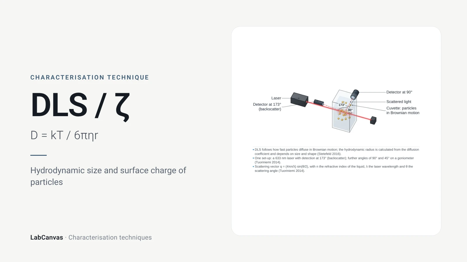
DLS and zeta potential explained: Brownian motion, Stokes–Einstein hydrodynamic size, intensity vs number distributions, PDI and colloidal stability.
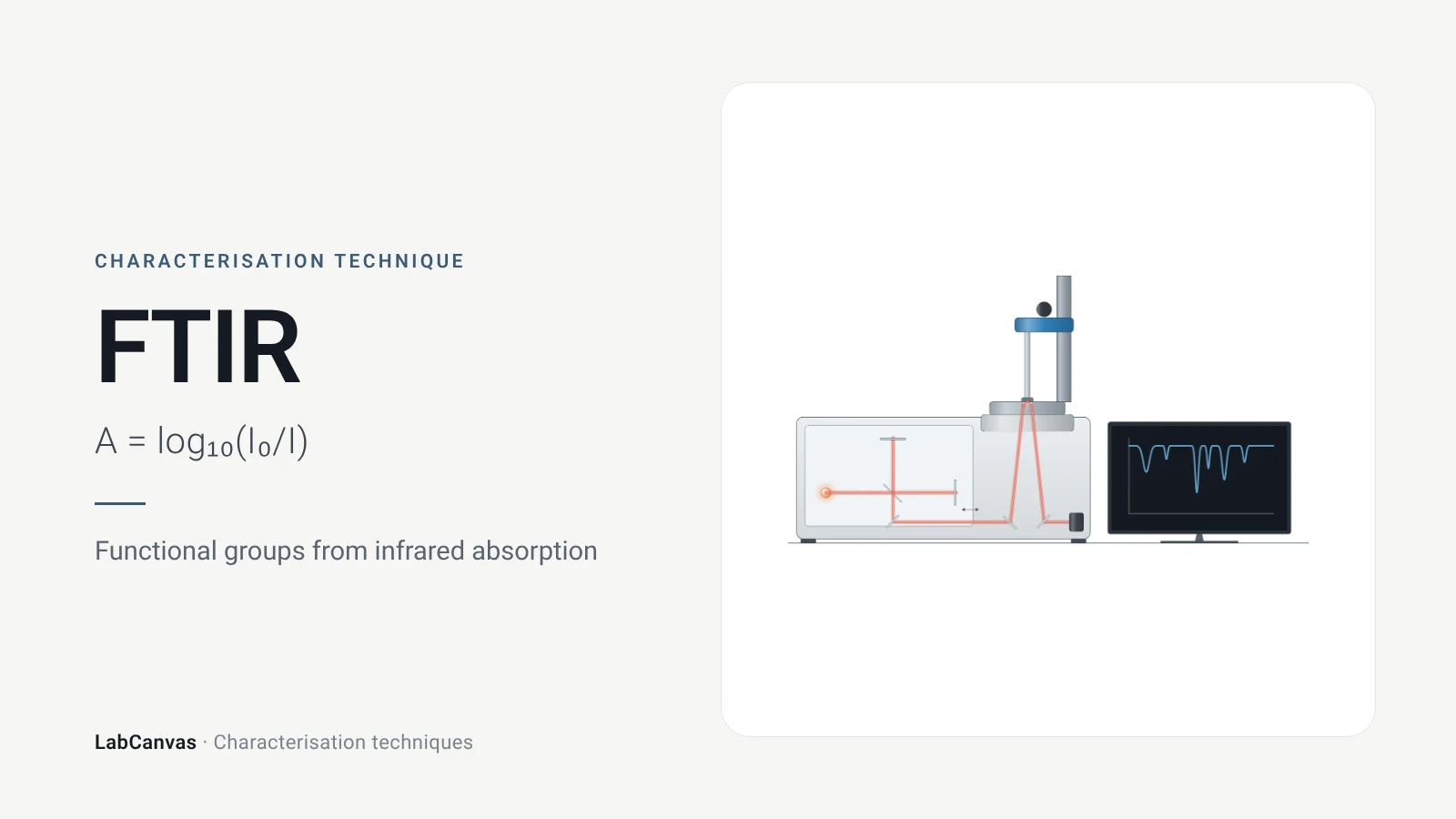
Fourier-transform infrared (FTIR) spectroscopy
FTIR spectroscopy explained: infrared absorption by bond vibrations, the interferometer and Fourier transform, wavenumber regions, ATR and reading bands.
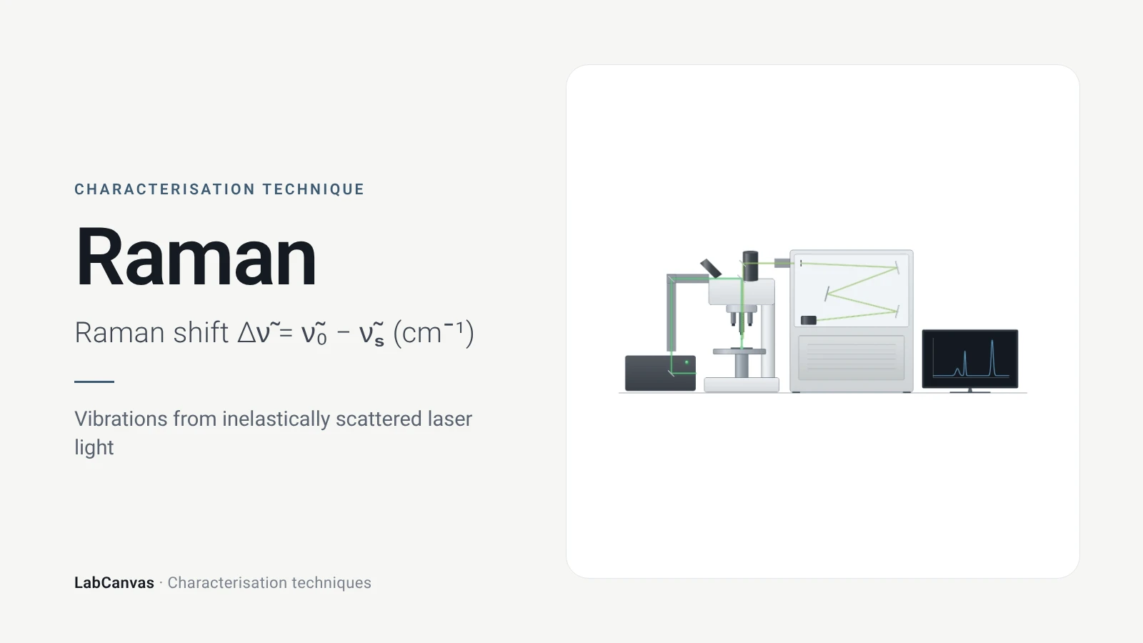
Raman spectroscopy
Raman spectroscopy explained: inelastic laser scattering, Raman shift, Stokes lines, IR complementarity, graphene D, G and 2D bands, lasers, fluorescence.
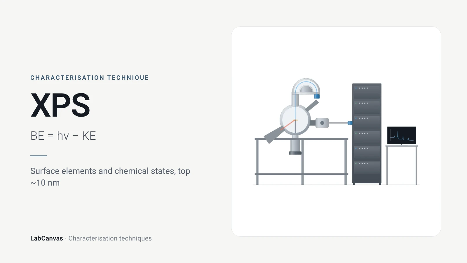
X-ray photoelectron spectroscopy (XPS)
XPS explained: binding energy, 2–10 nm surface sensitivity, survey vs high-resolution spectra, chemical shifts, C 1s charge referencing and depth profiling.
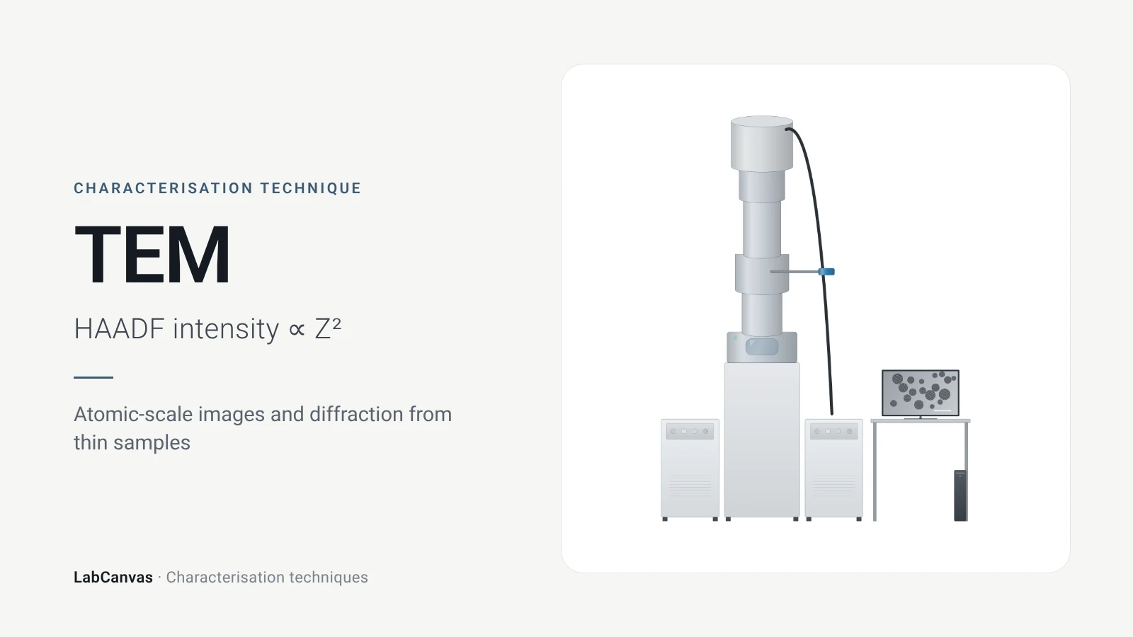
Transmission electron microscopy (TEM)
How TEM works: bright field, HRTEM lattice images, SAED diffraction, STEM-HAADF Z-contrast, EDS/EELS, sample thickness and beam damage of MOFs.
More on LabCanvas
- All characterisation techniques: XRD, XPS, BET, SEM, TEM, NMR, FTIR, Raman and more, explained with cited sources
- Graphical abstract sizes and templates: ACS, Wiley, Angewandte, RSC, Elsevier and Cell Press, with templates at the right size
- Tauc plot band gap calculator: Free tool
- Materials explained: MOFs, COFs, 2D materials, perovskites, batteries and zeolites, with cited facts
- Journal figure size guide: Column widths and resolutions for 38 journals
Frequently asked questions
What is UV–vis spectroscopy used for?
UV–vis measures how much ultraviolet and visible light a sample absorbs. It is used to measure concentration through the Beer–Lambert law, to find the optical band gap of semiconductors from a Tauc plot and to follow the plasmon band of metal nanoparticles (Mayerhöfer et al. 2019; Escobedo-Morales et al. 2019; Haiss et al. 2007).
What is the Beer–Lambert law?
Absorbance is proportional to concentration and path length: A = εcl, where ε is the molar attenuation coefficient. It holds for monochromatic light and non-interacting absorbers and fails with poor spectral resolution, detector nonlinearity, chemical interactions or scattering (Mayerhöfer et al. 2019).
How do you calculate the band gap from a Tauc plot?
Plot (αhν)^(1/n) against photon energy hν, with n = 1/2 for a direct allowed and 2 for an indirect allowed transition, fit a straight line to the steep absorption edge and read Eg where the line meets the energy axis (Escobedo-Morales et al. 2019). The free LabCanvas Tauc plot band gap calculator does the conversion and the fit.
How do you measure the band gap of a powder?
Measure diffuse reflectance against a PTFE or BaSO₄ standard, convert it to the Kubelka–Munk function F(R∞) = (1 − R∞)²/2R∞ and use F(R∞) in place of α in the Tauc plot; transmission does not work because powders scatter (Escobedo-Morales et al. 2019).
What is the difference between a direct and an indirect band gap in a Tauc plot?
Only the exponent changes: for a direct allowed transition you plot (αhν)², for an indirect allowed transition (αhν)^(1/2) (Escobedo-Morales et al. 2019). Using the wrong one gives a wrong gap.
Why is a gold nanoparticle solution red?
Dispersed gold nanoparticles have a localised surface plasmon band near 520 nm. When they aggregate the band red-shifts and broadens and the colour turns from wine-red to purple or blue (Wang et al. 2026).
Can UV–vis give nanoparticle size?
For spherical gold nanoparticles of 5 to 100 nm, yes: the plasmon band can be used to determine both size and concentration (Haiss et al. 2007). For other particles, or to check aggregation, use DLS or TEM.
Why is my Tauc plot band gap wrong?
Common causes are the wrong exponent, absorption below the gap that bends the baseline (Zhong et al. 2023), measuring a powder in transmission instead of diffuse reflectance, or a second absorbing phase, which makes the axis intercept underestimate the gap (Escobedo-Morales et al. 2019).
References
- T. G. Mayerhöfer, A. V. Pipa, J. Popp. Beer's law—why integrated absorbance depends linearly on concentration. ChemPhysChem 2019, 20, 2748–2753. doi:10.1002/cphc.201900787
- A. Escobedo-Morales, I. I. Ruiz-López, M. de L. Ruiz-Peralta, L. Tepech-Carrillo, M. Sánchez-Cantú, J. E. Moreno-Orea. Automated method for the determination of the band gap energy of pure and mixed powder samples using diffuse reflectance spectroscopy. Heliyon 2019, 5, e01505. doi:10.1016/j.heliyon.2019.e01505
- H. Zhong et al.. Idealizing Tauc plot for accurate bandgap determination of semiconductor with ultraviolet–visible spectroscopy: a case study for cubic boron arsenide. J. Phys. Chem. Lett. 2023, 14, 6702–6708. doi:10.1021/acs.jpclett.3c01416
- S. K. Suram, P. F. Newhouse, J. M. Gregoire. High throughput light absorber discovery, part 1: an algorithm for automated Tauc analysis. ACS Comb. Sci. 2016, 18, 673–681. doi:10.1021/acscombsci.6b00053
- L. Li et al.. Study on the origin of linear deviation with the Beer–Lambert law in absorption spectroscopy by measuring sulfur dioxide. Spectrochim. Acta A 2022, 275, 121192. doi:10.1016/j.saa.2022.121192
- W. Haiss, N. T. K. Thanh, J. Aveyard, D. G. Fernig. Determination of size and concentration of gold nanoparticles from UV–vis spectra. Anal. Chem. 2007, 79, 4215–4221. doi:10.1021/ac0702084
- S. Wang et al.. A review of aggregation-based colorimetric and SERS sensing of metal ions utilizing Au/Ag nanoparticles. Biosensors 2026, 16, 110. doi:10.3390/bios16020110
- A. Wishard, B. C. Gibb. Dynamic light scattering – an all-purpose guide for the supramolecular chemist. Supramol. Chem. 2019, 31, 608–615. doi:10.1080/10610278.2019.1629438
- M. Danaei et al.. Impact of particle size and polydispersity index on the clinical applications of lipidic nanocarrier systems. Pharmaceutics 2018, 10, 57. doi:10.3390/pharmaceutics10020057
Draw UV–vis spectroscopy figures for your paper
LabCanvas is a browser workspace for scientific figures: instruments with their beam and light paths, editable data plots, crystal structures, graphs and graphical abstracts at journal sizes.
Draw UV–vis spectroscopy in LabCanvas