Atomic force microscopy (AFM): how it works, contact vs tapping mode and height profiles
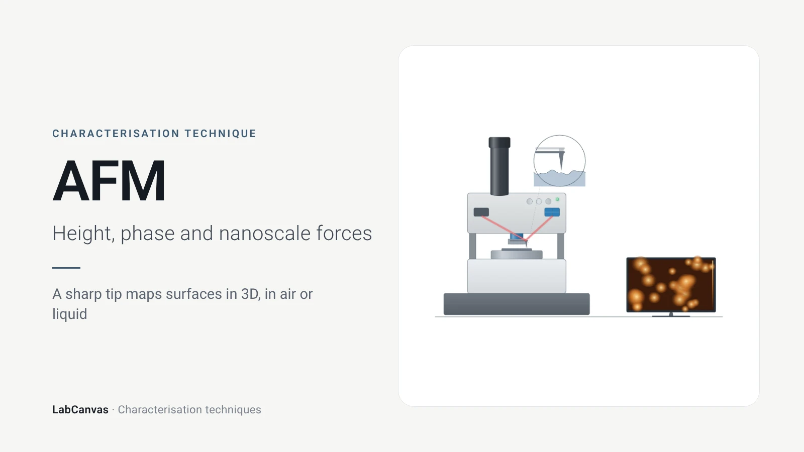
Atomic force microscopy (AFM) maps a surface by scanning a nanometre-sharp tip on a flexible cantilever across it; a laser reflected off the cantilever onto a photodiode records its bending, and a feedback loop moves the scanner up and down to keep the tip–sample interaction constant, so the scanner height becomes a 3D topographic map (Joo et al. 2025). It reaches 1–10 nm lateral and sub-nanometre vertical resolution without vacuum, which makes it the standard way to measure the thickness of 2D flakes, roughness and step heights, and its special modes map mechanical, electrical and magnetic properties (Joo et al. 2025).
Contents
Atomic force microscopy (AFM) at a glance
| Probe | Ultra-sharp tip, a few nanometres in apex radius, on a flexible cantilever (Joo et al. 2025) |
|---|---|
| Signal measured | Cantilever deflection or oscillation, read by a laser reflected onto a position-sensitive photodiode; topography from the Z-scanner height (Joo et al. 2025) |
| Main information | True 3D surface topography, roughness and step heights; mechanical, electrical and magnetic properties in special modes (Joo et al. 2025) |
| Lateral resolution | 1–10 nm typical (Joo et al. 2025) |
| Vertical resolution | Below 1 nm (Joo et al. 2025) |
| Scan range | X-Y piezo range 30–100 µm, Z about 10 µm, depending on model (Joo et al. 2025) |
| Environment | Ambient air, vacuum or liquid; no vacuum required (Joo et al. 2025) |
| Typical sample | Flat surfaces, films, flakes or particles fixed on a smooth substrate (Joo et al. 2025) |
| Imaging modes | Contact mode (constant deflection); non-contact and tapping modes (oscillating cantilever, constant amplitude or frequency shift) (Joo et al. 2025) |
| Monolayer heights measured | Graphene ~0.35 nm on deposition, ~0.8 nm weeks later (Sidorov et al. 2007); monolayer MoS₂ ~0.7 nm, reduced graphene oxide 0.4 nm (Sengottaiyan et al. 2025) |
| Invented | 1986, by Binnig, Quate and Gerber (Joo et al. 2025) |
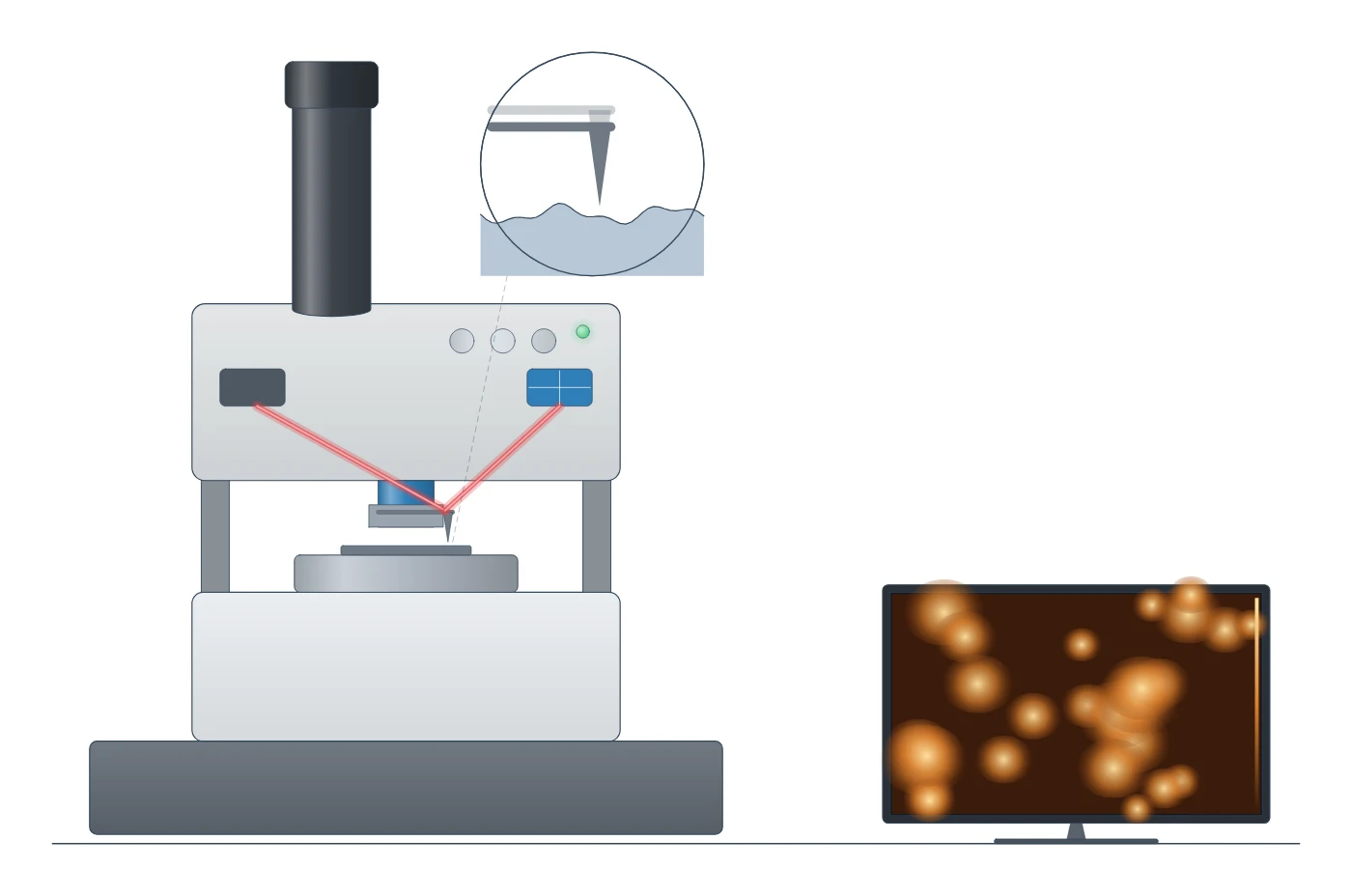
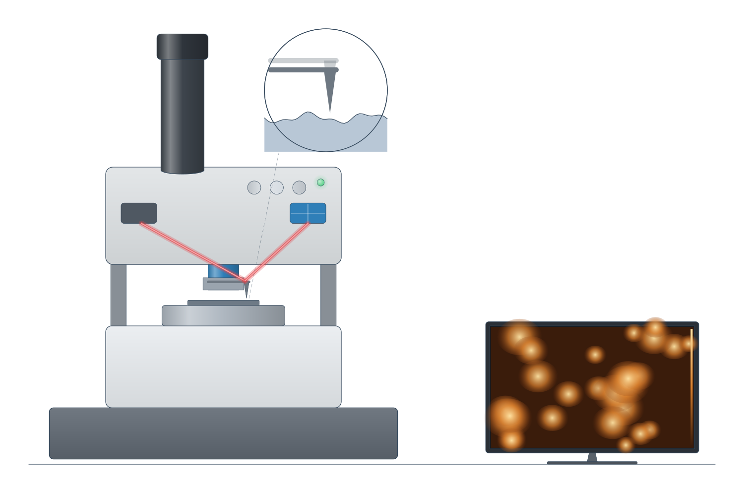
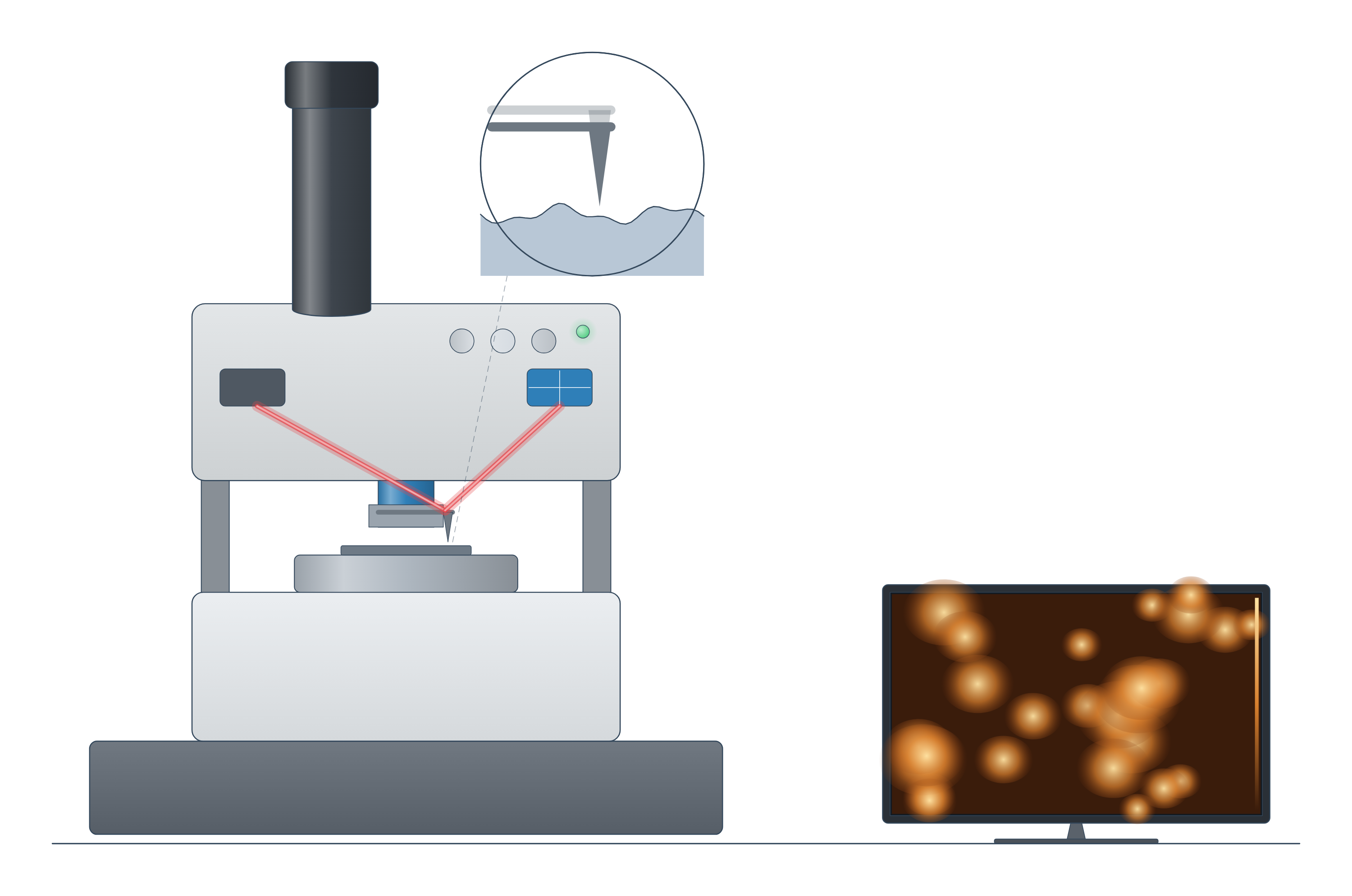
Atomic force microscopy (AFM) instrument drawing (high-resolution SVG)
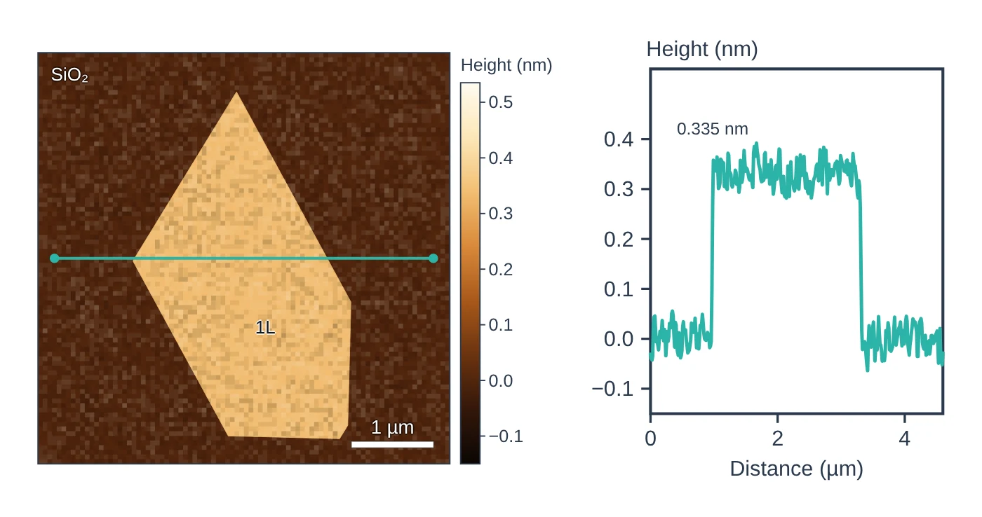
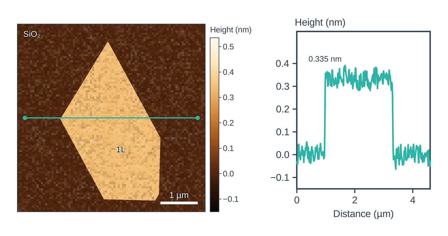
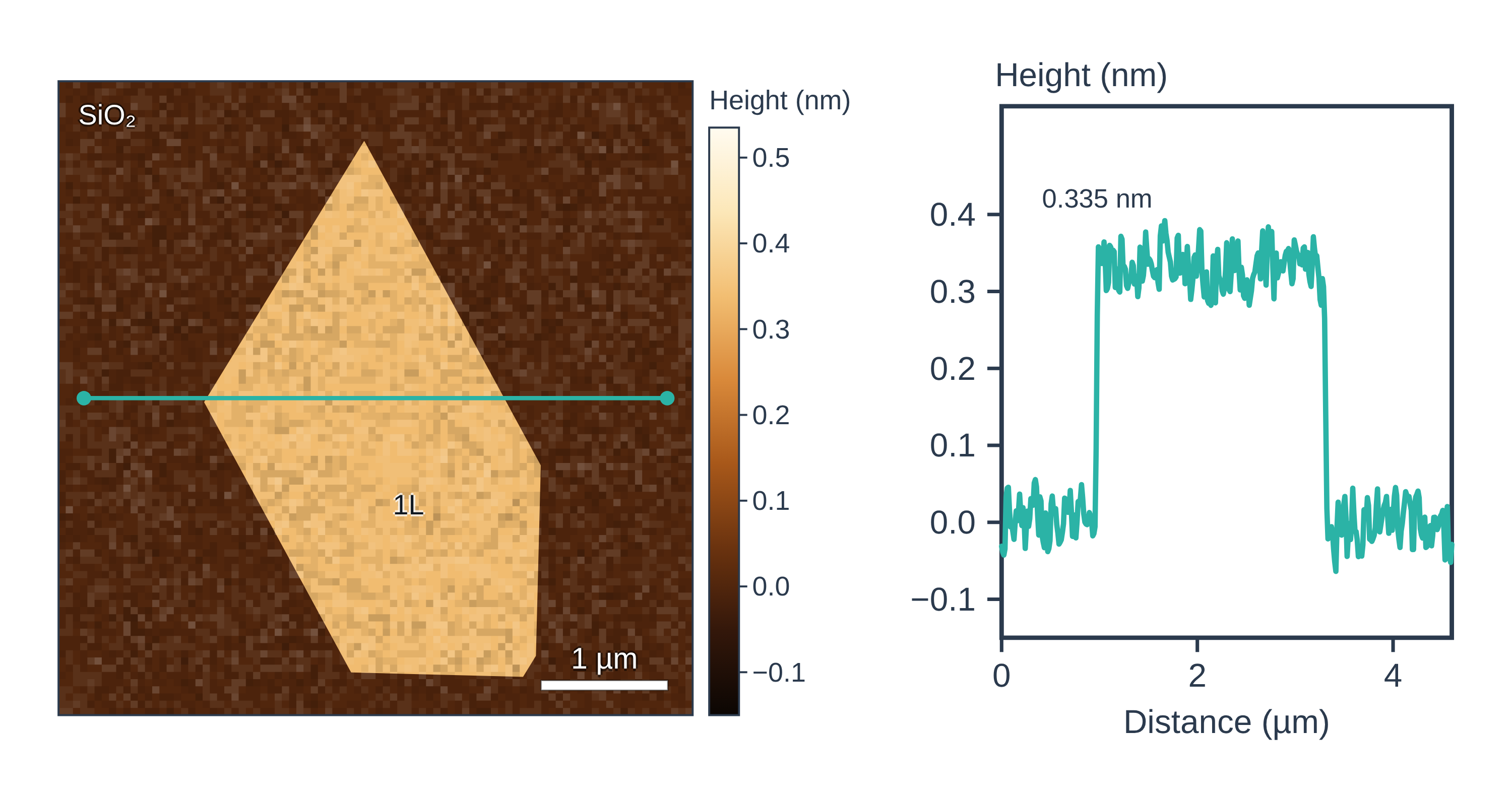
Atomic force microscopy (AFM) data: an example plot to edit
How AFM works
An AFM has no lenses. A flexible cantilever carries an ultra-sharp tip, a few nanometres in radius at its apex. A laser reflects off the back of the cantilever onto a position-sensitive photodiode split into quadrants: vertical bending of the cantilever moves the spot up or down (topography), and twisting moves it sideways (friction) (Joo et al. 2025).
Piezoelectric actuators scan the tip line by line over the sample (30–100 µm in X-Y, about 10 µm in Z), and a feedback loop raises or lowers the Z-scanner to keep the interaction at a chosen setpoint. The recorded Z-scanner height at each pixel is the topography image (Joo et al. 2025).
- Contact mode: the tip stays in contact and the feedback holds the cantilever deflection constant. The loading force is set by the cantilever spring constant k, the inverse optical lever sensitivity (InvOLS) and the setpoint, so F = k × InvOLS × setpoint. It is good for flat, rigid surfaces and for electrical modes, but the tip can damage soft or fragile samples (Joo et al. 2025).
- Non-contact and tapping (dynamic) modes: the cantilever oscillates near its resonance frequency and the feedback holds the oscillation amplitude (AM-AFM) or frequency shift (FM-AFM) constant. Non-contact mode works in the attractive-force regime and tapping mode in the repulsive regime, and these oscillating modes keep lateral forces that could distort the image to a minimum (Joo et al. 2025).
The same platform measures more than height: conductive AFM (current), Kelvin probe force microscopy (surface potential and work function), piezoresponse force microscopy (ferroelectric domains), magnetic force microscopy and electrochemical strain microscopy (ion motion) (Joo et al. 2025).
What the data looks like and how to read it
- Height image: a colour or grey scale of surface height. Read the colour bar, not the colours: the z-scale you choose can exaggerate or hide features (Joo et al. 2025).
- Height (line) profile: draw a line across a flake edge or step and read the height difference from the cross-section; height histograms show steps, terraces and coatings as separate peaks (Joo et al. 2025). This is how 2D flake thickness is measured: about 0.7 nm for monolayer MoS₂ and 0.4 nm for reduced graphene oxide in one study (Sengottaiyan et al. 2025).
- Deflection or amplitude image: the error signal of the feedback; it mostly highlights steep slopes and edges (Joo et al. 2025).
- Phase image (dynamic modes): the lag between drive and response, sensitive to viscosity, adhesion and elasticity, so it separates components of a blend or composite (Joo et al. 2025).
Sample preparation
- Deposited particles and piled structures can drift under the tip in contact mode; non-contact mode with a carefully set setpoint and scan rate can give more accurate results (Joo et al. 2025).
- Choose the mode for the sample: contact mode for flat, rigid surfaces and electrical contact; non-contact or tapping mode for soft or fragile samples (Joo et al. 2025).
- Calibrate the cantilever spring constant and InvOLS before quantitative force work, and use a reference material (gold or HOPG for the KPFM tip work function; a PS–LDPE sample for nanoindentation) (Joo et al. 2025).
- Reduce vibration and electrical noise with isolation; humidity and temperature also affect results (Joo et al. 2025).
What AFM tells you about materials
- 2D materials: layer number and thickness of graphene, MoS₂, h-BN and graphene oxide flakes from height profiles (Sengottaiyan et al. 2025); AFM and STM fold heights showed that folds in CVD graphene are three layers thick (Huang et al. 2018). KPFM and electrostatic force microscopy also map surface potential and carrier density in monolayer WS₂ (Joo et al. 2025).
- Battery materials: operando electrochemical AFM has followed solid electrolyte interphase growth on graphite anodes during cycling, and electrochemical strain microscopy maps local ion mobility (Joo et al. 2025). See the battery materials hub.
- Films and coatings: height histograms give uniformity, roughness and thickness variations of thin films, such as the perovskite films, and PFM maps ferroelectric domains in oxide heterostructures (Joo et al. 2025).
- Polymers and composites: phase and modulus maps separate stiff and soft phases (Joo et al. 2025).
AFM complements SEM and TEM, which give limited height information and need vacuum (Joo et al. 2025), and spectroscopies such as Raman. Compare all methods on the characterisation techniques page.
Common mistakes and limits
- Tip convolution. The tip cannot follow steep walls, so features look broader than they are; compare trace and retrace, rescan after rotating the sample, and use sharper or high-aspect-ratio tips (Joo et al. 2025).
- Trusting a single monolayer height. Measured heights depend on the substrate, adsorbed layers and imaging conditions: one graphene sheet measured ~0.35 nm on deposition and ~0.8 nm a few weeks later (Sidorov et al. 2007). The imaging mode matters too: on a polystyrene–polyethylene blend, contact and non-contact height images differ because the two polymers differ in stiffness (Joo et al. 2025).
- Processing artefacts. Line-by-line flattening can create stripes next to tall particles unless they are masked; plane fitting can distort genuinely tilted surfaces; filtered images should not be used for measurements (Joo et al. 2025).
- Thermal drift and noise. Drift distorts the slow-scan axis on long scans, and building vibrations add periodic noise (Joo et al. 2025).
- Small field of view and slow scans. The X-Y scan range is 30–100 µm and scanning is slow, so collect several areas and treat each image statistically (Joo et al. 2025).
- Damaging soft samples with too high a setpoint in contact mode (Joo et al. 2025).
How to draw the AFM setup and data in LabCanvas
A good AFM figure shows the cantilever and tip over the sample, the laser reflecting onto the quadrant photodiode and the feedback loop to the piezo scanner, next to a height image with a line marked across a flake and the matching height profile. In LabCanvas the figure editor Library has the AFM as an editable object, including a cutaway of the laser light path from cantilever to photodiode, and an editable data plot for the height profile. You can label the step height, add a scale bar and colour bar, and export the figure for a methods section or a graphical abstract.
AFM compared with SEM and TEM
| Technique | What it measures | Resolution | Sample damage | Vacuum | In situ | Source |
|---|---|---|---|---|---|---|
| AFM | Topography (true height) plus mechanical, electrical, magnetic properties | 1–10 nm lateral, below 1 nm vertical | Subtle | Not required | Available | Joo et al. 2025 |
| SEM | Surface morphology; composition with EDS | Nanometre scale | Moderate | Required (low vacuum possible) | Challenging | Joo et al. 2025 |
| TEM | Nanostructure, atomic and crystal structure; composition with EDS | Sub-nanometre | Profound | High vacuum | Challenging | Joo et al. 2025 |
Related techniques
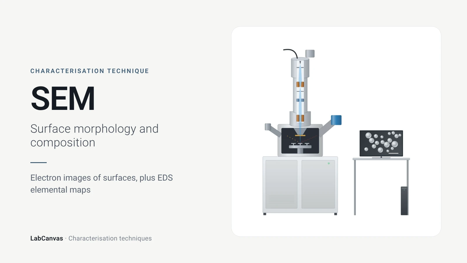
Scanning electron microscopy (SEM)
How SEM works: secondary vs backscattered electron images, EDS/EDX elemental analysis, resolution, sample coating, low-vacuum mode and common mistakes.
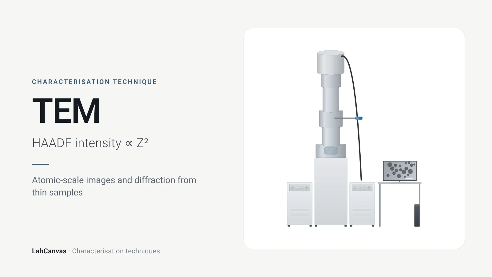
Transmission electron microscopy (TEM)
How TEM works: bright field, HRTEM lattice images, SAED diffraction, STEM-HAADF Z-contrast, EDS/EELS, sample thickness and beam damage of MOFs.
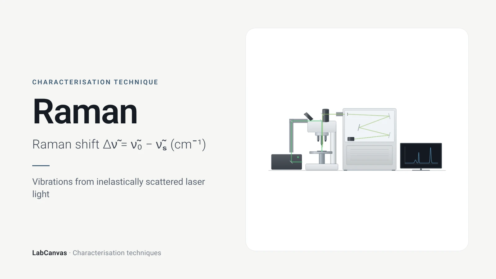
Raman spectroscopy
Raman spectroscopy explained: inelastic laser scattering, Raman shift, Stokes lines, IR complementarity, graphene D, G and 2D bands, lasers, fluorescence.
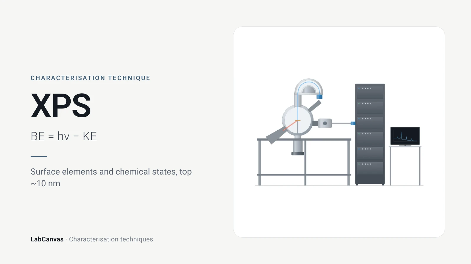
X-ray photoelectron spectroscopy (XPS)
XPS explained: binding energy, 2–10 nm surface sensitivity, survey vs high-resolution spectra, chemical shifts, C 1s charge referencing and depth profiling.
More on LabCanvas
- All characterisation techniques: XRD, XPS, BET, SEM, TEM, NMR, FTIR, Raman and more, explained with cited sources
- Graphical abstract sizes and templates: ACS, Wiley, Angewandte, RSC, Elsevier and Cell Press, with templates at the right size
- Materials explained: MOFs, COFs, 2D materials, perovskites, batteries and zeolites, with cited facts
- Journal figure size guide: Column widths and resolutions for 38 journals
Frequently asked questions
What is AFM used for?
AFM maps surface topography in 3D with sub-nanometre vertical resolution, measuring roughness, step heights and the thickness of 2D flakes, and special modes map mechanical, electrical and magnetic properties (Joo et al. 2025).
How does an AFM work?
A sharp tip on a flexible cantilever is scanned over the surface; a laser reflected off the cantilever onto a photodiode detects its bending, and a feedback loop moves the Z-scanner to keep the interaction constant, so the scanner height gives the topography (Joo et al. 2025).
What is the difference between contact mode and tapping mode AFM?
In contact mode the tip touches the surface and the deflection is held constant, which suits flat, rigid samples but can damage soft ones; in tapping mode the cantilever oscillates near resonance in the repulsive regime, which keeps lateral forces low and suits softer samples (Joo et al. 2025).
How do you measure the thickness of a 2D flake by AFM?
Draw a line profile across the flake edge in the height image and read the step between substrate and flake; monolayer MoS₂ measured about 0.7 nm this way (Sengottaiyan et al. 2025; Joo et al. 2025).
How thick is monolayer graphene in AFM?
One freshly deposited graphene sheet measured about 0.35 nm by AFM, but the same sheet measured about 0.8 nm a few weeks later, so AFM heights of monolayers depend on the sample history and should be checked with other methods (Sidorov et al. 2007).
What are common AFM artefacts?
Tip convolution that broadens features, thermal drift along the slow-scan axis, vibration noise and distortions introduced by flattening or filtering during image processing (Joo et al. 2025).
What is the resolution of AFM?
Typically 1–10 nm laterally and below 1 nm vertically, depending on the instrument, mode and sample (Joo et al. 2025).
AFM vs SEM: which should I use?
Use SEM for fast, large-area morphology and EDS composition; use AFM when you need true height, roughness or nanoscale properties, or must image in air or liquid without vacuum (Joo et al. 2025).
References
- S. Joo et al.. Atomic force microscopy for cross-disciplinary materials research. Small Methods 2025, 9, e2500514. doi:10.1002/smtd.202500514
- A. N. Sidorov et al.. Electrostatic deposition of graphene. Nanotechnology 2007, 18, 135301. doi:10.1088/0957-4484/18/13/135301
- C. Sengottaiyan, K. Hirosawa, Y. Kurachi, M. Hara, M. Yoshimura. Investigating local electron transport dynamics in layer-dependent MoS₂/RGO heterostructures using conductive atomic force microscopy. ACS Appl. Mater. Interfaces 2025, 17, 34294–34303. doi:10.1021/acsami.5c09185
- M. Huang et al.. Highly oriented monolayer graphene grown on a Cu/Ni(111) alloy foil. ACS Nano 2018, 12, 6117–6127. doi:10.1021/acsnano.8b02444
Draw Atomic force microscopy (AFM) figures for your paper
LabCanvas is a browser workspace for scientific figures: instruments with their beam and light paths, editable data plots, crystal structures, graphs and graphical abstracts at journal sizes.
Draw Atomic force microscopy (AFM) in LabCanvas