TikZ neural network diagrams: perceptron, MLP, CNN, LSTM and transformer
Quick answer
\foreach loops and connect consecutive layers with a third: with the layer sizes in a list, \foreach \n [count=\l] in {3,5,5,2} places \n neurons in column \l, centred with the y coordinate (\n+1)/2 − \i, and names each one (N\l-\i). The loop key remember=\n as \prev keeps the size of the previous layer, so every neuron of layer \l−1 can be joined to every neuron of layer \l. Change the list and the whole network redraws. CNNs, LSTMs and transformers are built from the same pieces (nodes, styles and arrows); the code for each is below.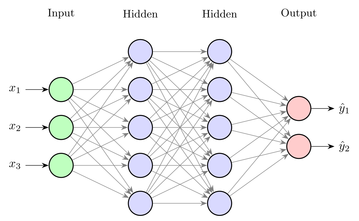
\usepackage{tikz} \usetikzlibrary{arrows.meta}\begin{tikzpicture}[x=2.3cm, y=1.1cm, >={Stealth[length=2mm]},
neuron/.style={circle, draw, thick, minimum size=7mm, inner sep=0pt}]
% one entry per layer: number of neurons / fill colour / label
\foreach \n/\c/\name [count=\l, remember=\n as \prev (initially 0)] in
{3/green!25/Input, 5/blue!15/Hidden, 5/blue!15/Hidden, 2/red!20/Output} {
\foreach \i in {1,...,\n}
\node[neuron, fill=\c] (N\l-\i) at (\l, {(\n+1)/2 - \i}) {};
\node[font=\small] at (\l, 3) {\name};
% connect every neuron of the previous layer to every neuron of this one
\ifnum\l>1
\pgfmathtruncatemacro\k{\l - 1}
\foreach \i in {1,...,\prev}
\foreach \j in {1,...,\n}
\draw[->, gray] (N\k-\i) -- (N\l-\j);
\fi
}
\foreach \i in {1,2,3} \draw[<-] (N1-\i) -- ++(-0.45,0) node[left] {$x_\i$};
\foreach \i in {1,2} \draw[->] (N4-\i) -- ++(0.45,0) node[right] {$\hat y_\i$};
\end{tikzpicture}Full document
\documentclass[border=4pt]{standalone}
\usepackage{tikz}
\usetikzlibrary{arrows.meta}
\begin{document}
\begin{tikzpicture}[x=2.3cm, y=1.1cm, >={Stealth[length=2mm]},
    neuron/.style={circle, draw, thick, minimum size=7mm, inner sep=0pt}]
  % one entry per layer: number of neurons / fill colour / label
  \foreach \n/\c/\name [count=\l, remember=\n as \prev (initially 0)] in
      {3/green!25/Input, 5/blue!15/Hidden, 5/blue!15/Hidden, 2/red!20/Output} {
    \foreach \i in {1,...,\n}
      \node[neuron, fill=\c] (N\l-\i) at (\l, {(\n+1)/2 - \i}) {};
    \node[font=\small] at (\l, 3) {\name};
    % connect every neuron of the previous layer to every neuron of this one
    \ifnum\l>1
      \pgfmathtruncatemacro\k{\l - 1}
      \foreach \i in {1,...,\prev}
        \foreach \j in {1,...,\n}
          \draw[->, gray] (N\k-\i) -- (N\l-\j);
    \fi
  }
  \foreach \i in {1,2,3} \draw[<-] (N1-\i) -- ++(-0.45,0) node[left] {$x_\i$};
  \foreach \i in {1,2}   \draw[->] (N4-\i) -- ++(0.45,0) node[right] {$\hat y_\i$};
\end{tikzpicture}
\end{document}Contents
A fully connected network from a list of layer sizes
The picture at the top is one loop over the layers. Each entry of the list is size/colour/label, read into \n/\c/\name; count=\l numbers the layers from 1 and remember=\n as \prev (initially 0) makes the previous layer’s size available in the next pass. Inside, a second loop places the neurons: column \l (with x=2.3cm on the picture, the columns are 2.3 cm apart) and rows (\n+1)/2 − \i, which centres every layer on the axis whatever its size. Naming the nodes (N\l-\i) makes the connections easy: a third and fourth loop draw (N\k-\i) -- (N\l-\j) for all pairs, where \k = \l − 1 is computed with \pgfmathtruncatemacro (an integer, so that the name is N1-2 and not N1.0-2). The lines end at the circles’ borders automatically.
Two details: the first layer has no predecessor, so the connections are wrapped in \ifnum\l>1 … \fi (without it TikZ looks for a node N0-1, see the errors below); and each pass of \foreach is a TeX group, so a macro defined in one pass is gone in the next, which is why the previous size travels through remember. Inputs and outputs are added after the loop as short arrows from the named nodes. For a deeper network, add entries to the list; for many neurons, draw a few and a \vdots node in between.
A single neuron: the perceptron
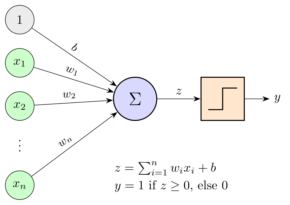
A neuron computes a weighted sum of its inputs plus a bias, z = Σwixi + b, and passes it through an activation function. Rosenblatt’s perceptron uses a step, y = 1 if z ≥ 0 and 0 otherwise, drawn here as three line segments inside the activation box; for a sigmoid or ReLU neuron, draw that curve instead, for example a short plot. The bias is shown as the weight of a constant input 1, the usual trick that makes it look like any other weight.
The weight labels sit on their edges with node[pos=0.45, above, sloped]: sloped turns the text along the line and pos moves it along, which keeps labels on converging edges apart. The xn input and the \vdots stand for any number of inputs.
\usepackage{tikz} \usetikzlibrary{arrows.meta, positioning}\begin{tikzpicture}[>={Stealth[length=2mm]},
input/.style={circle, draw, fill=green!20, minimum size=8mm, inner sep=0pt}]
% inputs x_1 ... x_n and the constant 1 that carries the bias b
\node[input, fill=gray!15] (b) at (0, 2.4) {$1$};
\node[input] (x1) at (0, 1.2) {$x_1$};
\node[input] (x2) at (0, 0) {$x_2$};
\node at (0,-1) {$\vdots$};
\node[input] (xn) at (0,-2.2) {$x_n$};
% weighted sum and step activation
\node[circle, draw, thick, fill=blue!15, minimum size=12mm] (sum) at (3.2,0.2) {\Large$\Sigma$};
\node[draw, thick, fill=orange!20, minimum size=12mm, right=12mm of sum] (act) {};
\draw[thick] ([shift={(-4mm,-3mm)}]act.center) -- ++(4mm,0) -- ++(0,6mm) -- ++(4mm,0);
\foreach \i in {1,2,n}
\draw[->] (x\i) -- node[pos=0.45, above, sloped, font=\small] {$w_{\i}$} (sum);
\draw[->] (b) -- node[pos=0.45, above, sloped, font=\small] {$b$} (sum);
\draw[->] (sum) -- node[above] {$z$} (act);
\draw[->] (act) -- ++(1.3,0) node[right] {$y$};
\node[below=10mm of sum, xshift=10mm, align=left] {%
$z = \sum_{i=1}^{n} w_i x_i + b$\\[2pt]
$y = 1$ if $z \ge 0$, else $0$};
\end{tikzpicture}Full document
\documentclass[border=4pt]{standalone}
\usepackage{tikz}
\usetikzlibrary{arrows.meta, positioning}
\begin{document}
\begin{tikzpicture}[>={Stealth[length=2mm]},
    input/.style={circle, draw, fill=green!20, minimum size=8mm, inner sep=0pt}]
  % inputs x_1 ... x_n and the constant 1 that carries the bias b
  \node[input, fill=gray!15] (b)  at (0, 2.4) {$1$};
  \node[input]               (x1) at (0, 1.2) {$x_1$};
  \node[input]               (x2) at (0, 0)   {$x_2$};
  \node                           at (0,-1)   {$\vdots$};
  \node[input]               (xn) at (0,-2.2) {$x_n$};
  % weighted sum and step activation
  \node[circle, draw, thick, fill=blue!15, minimum size=12mm] (sum) at (3.2,0.2) {\Large$\Sigma$};
  \node[draw, thick, fill=orange!20, minimum size=12mm, right=12mm of sum] (act) {};
  \draw[thick] ([shift={(-4mm,-3mm)}]act.center) -- ++(4mm,0) -- ++(0,6mm) -- ++(4mm,0);
  \foreach \i in {1,2,n}
    \draw[->] (x\i) -- node[pos=0.45, above, sloped, font=\small] {$w_{\i}$} (sum);
  \draw[->] (b) -- node[pos=0.45, above, sloped, font=\small] {$b$} (sum);
  \draw[->] (sum) -- node[above] {$z$} (act);
  \draw[->] (act) -- ++(1.3,0) node[right] {$y$};
  \node[below=10mm of sum, xshift=10mm, align=left] {%
    $z = \sum_{i=1}^{n} w_i x_i + b$\\[2pt]
    $y = 1$ if $z \ge 0$, else $0$};
\end{tikzpicture}
\end{document}Labelled weights and activations
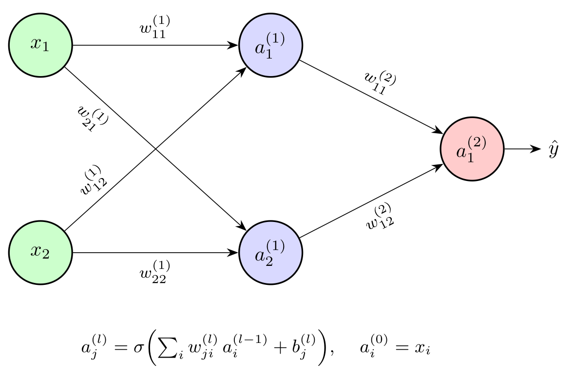
For a figure that explains the maths, label every weight and activation. A common notation is w(l)ji for the weight from neuron i of layer l − 1 to neuron j of layer l, and a(l)j = σ(Σi w(l)ji a(l−1)i + b(l)j) for its activation; writing the activation inside the node needs a larger minimum size (11 mm here).
The crossing edges are where labels collide. Put those labels near the start of their edges (pos=0.22) and on the side facing the empty space: for the edge going down, below (with sloped, “below” is the right-hand side of the direction of travel), for the edge going up, above. A w style holds the common keys (font=\footnotesize, sloped, above), and individual edges override only what differs.
\usepackage{tikz} \usetikzlibrary{arrows.meta}\begin{tikzpicture}[>={Stealth[length=2mm]},
neuron/.style={circle, draw, thick, minimum size=11mm, inner sep=0pt},
w/.style={font=\footnotesize, sloped, above}]
\node[neuron, fill=green!20] (x1) at (0, 1.8) {$x_1$};
\node[neuron, fill=green!20] (x2) at (0,-1.8) {$x_2$};
\node[neuron, fill=blue!15] (h1) at (4, 1.8) {$a^{(1)}_1$};
\node[neuron, fill=blue!15] (h2) at (4,-1.8) {$a^{(1)}_2$};
\node[neuron, fill=red!20] (y) at (7.5, 0) {$a^{(2)}_1$};
% w^{(l)}_{ji}: from neuron i of layer l-1 to neuron j of layer l
\draw[->] (x1) -- node[w] {$w^{(1)}_{11}$} (h1);
\draw[->] (x1) -- node[w, pos=0.22, below] {$w^{(1)}_{21}$} (h2);
\draw[->] (x2) -- node[w, pos=0.22] {$w^{(1)}_{12}$} (h1);
\draw[->] (x2) -- node[w, below] {$w^{(1)}_{22}$} (h2);
\draw[->] (h1) -- node[w] {$w^{(2)}_{11}$} (y);
\draw[->] (h2) -- node[w, below] {$w^{(2)}_{12}$} (y);
\draw[->] (y) -- ++(1.2,0) node[right] {$\hat y$};
\node[below=6mm, font=\small] at (3.75,-2.4) {%
$a^{(l)}_j = \sigma\Bigl(\sum_i w^{(l)}_{ji}\, a^{(l-1)}_i + b^{(l)}_j\Bigr)$, \quad $a^{(0)}_i = x_i$};
\end{tikzpicture}Full document
\documentclass[border=4pt]{standalone}
\usepackage{tikz}
\usetikzlibrary{arrows.meta}
\begin{document}
\begin{tikzpicture}[>={Stealth[length=2mm]},
    neuron/.style={circle, draw, thick, minimum size=11mm, inner sep=0pt},
    w/.style={font=\footnotesize, sloped, above}]
  \node[neuron, fill=green!20] (x1) at (0, 1.8)  {$x_1$};
  \node[neuron, fill=green!20] (x2) at (0,-1.8)  {$x_2$};
  \node[neuron, fill=blue!15]  (h1) at (4, 1.8)  {$a^{(1)}_1$};
  \node[neuron, fill=blue!15]  (h2) at (4,-1.8)  {$a^{(1)}_2$};
  \node[neuron, fill=red!20]   (y)  at (7.5, 0)  {$a^{(2)}_1$};
  % w^{(l)}_{ji}: from neuron i of layer l-1 to neuron j of layer l
  \draw[->] (x1) -- node[w]           {$w^{(1)}_{11}$} (h1);
  \draw[->] (x1) -- node[w, pos=0.22, below] {$w^{(1)}_{21}$} (h2);
  \draw[->] (x2) -- node[w, pos=0.22]        {$w^{(1)}_{12}$} (h1);
  \draw[->] (x2) -- node[w, below]    {$w^{(1)}_{22}$} (h2);
  \draw[->] (h1) -- node[w]           {$w^{(2)}_{11}$} (y);
  \draw[->] (h2) -- node[w, below]    {$w^{(2)}_{12}$} (y);
  \draw[->] (y) -- ++(1.2,0) node[right] {$\hat y$};
  \node[below=6mm, font=\small] at (3.75,-2.4) {%
    $a^{(l)}_j = \sigma\Bigl(\sum_i w^{(l)}_{ji}\, a^{(l-1)}_i + b^{(l)}_j\Bigr)$, \quad $a^{(0)}_i = x_i$};
\end{tikzpicture}
\end{document}CNN diagrams: feature maps as pseudo-3D boxes
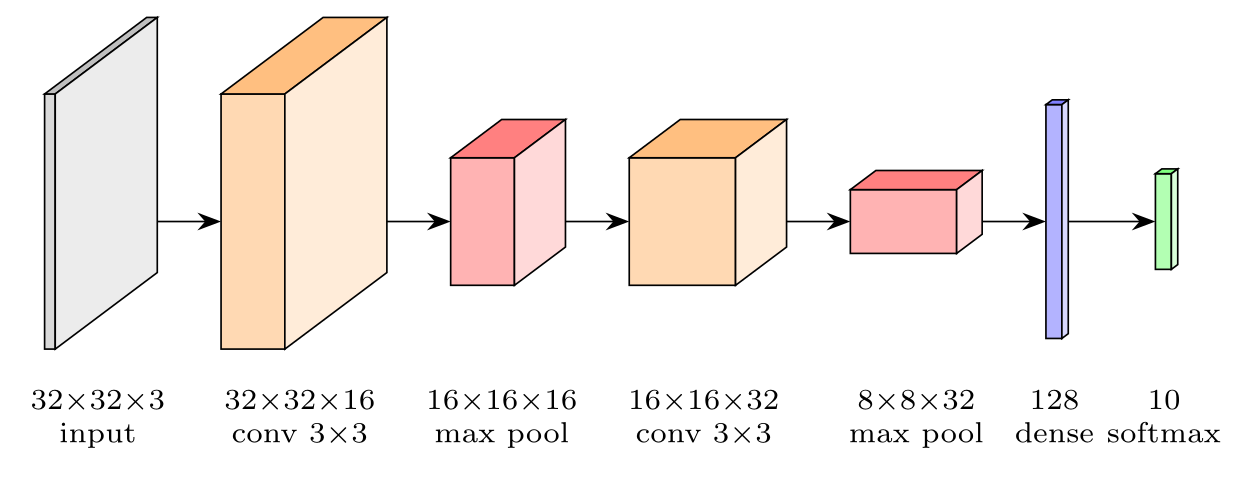
CNN figures show each layer’s output as a box: height and depth for the spatial size, thickness for the number of channels. The box is a pic with four arguments, defined with pics/fmap/.style n args={4}{code={…}} and used as \pic at (1.66,0) {fmap={0.6}{2.4}{2.4}{orange}};. It draws three faces: the front rectangle, then the top and the side as parallelograms receding at the same oblique offset, (0.4, 0.3) times the depth, in three shades of one colour so that the box reads as solid. This is an oblique sketch, not a true 3D projection, which is what such figures conventionally use.
The network shown is a small classifier for 32×32 colour images: a 3×3 convolution with padding keeps 32×32 and makes 16 channels, 2×2 max pooling halves the size, a second convolution gives 32 channels, a second pooling 8×8, then a dense layer of 128 and a softmax over 10 classes. The box sizes follow the tensor shapes roughly. The arrows are drawn first, so the boxes cover their ends.
\usepackage{tikz} \usetikzlibrary{arrows.meta}\begin{tikzpicture}[x=0.9cm, y=0.9cm, >={Stealth[length=2mm]}, font=\scriptsize,
% a feature map as a box: #1 thickness (channels), #2 height, #3 depth, #4 colour
pics/fmap/.style n args={4}{code={
\draw[fill=#4!30] (0,{-#2/2}) rectangle (#1,{#2/2});
\draw[fill=#4!50] (0,{#2/2}) -- ++({0.4*#3},{0.3*#3}) -- ++(#1,0)
-- ++({-0.4*#3},{-0.3*#3}) -- cycle;
\draw[fill=#4!15] (#1,{-#2/2}) -- ++({0.4*#3},{0.3*#3}) -- ++(0,#2)
-- ++({-0.4*#3},{-0.3*#3}) -- cycle;
}}]
% arrows first, so that the boxes cover their ends
\foreach \a/\b in {0.1/1.66, 2.26/3.82, 4.42/5.5, 6.5/7.58, 8.58/9.42, 9.57/10.45}
\draw[->] (\a,0) -- (\b,0);
\pic at (0,0) {fmap={0.1}{2.4}{2.4}{gray}}; % 32 x 32 x 3
\pic at (1.66,0) {fmap={0.6}{2.4}{2.4}{orange}}; % 32 x 32 x 16
\pic at (3.82,0) {fmap={0.6}{1.2}{1.2}{red}}; % 16 x 16 x 16
\pic at (5.5,0) {fmap={1.0}{1.2}{1.2}{orange}}; % 16 x 16 x 32
\pic at (7.58,0) {fmap={1.0}{0.6}{0.6}{red}}; % 8 x 8 x 32
\pic at (9.42,0) {fmap={0.15}{2.2}{0.15}{blue}}; % 128
\pic at (10.45,0) {fmap={0.15}{0.9}{0.15}{green}}; % 10
\foreach \x/\t in {0.5/{32$\times$32$\times$3\\input}, 2.4/{32$\times$32$\times$16\\conv 3$\times$3},
4.3/{16$\times$16$\times$16\\max pool}, 6.2/{16$\times$16$\times$32\\conv 3$\times$3},
8.2/{8$\times$8$\times$32\\max pool}, 9.5/{128\\dense}, 10.53/{10\\softmax}}
\node[align=center, anchor=north] at (\x,-1.45) {\t};
\end{tikzpicture}Full document
\documentclass[border=4pt]{standalone}
\usepackage{tikz}
\usetikzlibrary{arrows.meta}
\begin{document}
\begin{tikzpicture}[x=0.9cm, y=0.9cm, >={Stealth[length=2mm]}, font=\scriptsize,
  % a feature map as a box: #1 thickness (channels), #2 height, #3 depth, #4 colour
  pics/fmap/.style n args={4}{code={
    \draw[fill=#4!30] (0,{-#2/2}) rectangle (#1,{#2/2});
    \draw[fill=#4!50] (0,{#2/2}) -- ++({0.4*#3},{0.3*#3}) -- ++(#1,0)
                      -- ++({-0.4*#3},{-0.3*#3}) -- cycle;
    \draw[fill=#4!15] (#1,{-#2/2}) -- ++({0.4*#3},{0.3*#3}) -- ++(0,#2)
                      -- ++({-0.4*#3},{-0.3*#3}) -- cycle;
  }}]
  % arrows first, so that the boxes cover their ends
  \foreach \a/\b in {0.1/1.66, 2.26/3.82, 4.42/5.5, 6.5/7.58, 8.58/9.42, 9.57/10.45}
    \draw[->] (\a,0) -- (\b,0);
  \pic at (0,0)     {fmap={0.1}{2.4}{2.4}{gray}};     % 32 x 32 x 3
  \pic at (1.66,0)  {fmap={0.6}{2.4}{2.4}{orange}};   % 32 x 32 x 16
  \pic at (3.82,0)  {fmap={0.6}{1.2}{1.2}{red}};      % 16 x 16 x 16
  \pic at (5.5,0)   {fmap={1.0}{1.2}{1.2}{orange}};   % 16 x 16 x 32
  \pic at (7.58,0)  {fmap={1.0}{0.6}{0.6}{red}};      %  8 x  8 x 32
  \pic at (9.42,0)  {fmap={0.15}{2.2}{0.15}{blue}};   % 128
  \pic at (10.45,0) {fmap={0.15}{0.9}{0.15}{green}};  % 10
  \foreach \x/\t in {0.5/{32$\times$32$\times$3\\input}, 2.4/{32$\times$32$\times$16\\conv 3$\times$3},
                     4.3/{16$\times$16$\times$16\\max pool}, 6.2/{16$\times$16$\times$32\\conv 3$\times$3},
                     8.2/{8$\times$8$\times$32\\max pool}, 9.5/{128\\dense}, 10.53/{10\\softmax}}
    \node[align=center, anchor=north] at (\x,-1.45) {\t};
\end{tikzpicture}
\end{document}Recurrent networks: an unrolled RNN and an LSTM cell
A recurrent network is usually drawn twice: folded, with the hidden state looping back into the cell, and unrolled, with one copy of the same cell per time step. The loop is a to[out=-10, in=10, looseness=1.8] curve between two anchors on the cell’s right side, and the unrolled copies come from a \foreach over the steps with {t-1} in braces so that the minus sign stays in the subscript. A plain (Elman) cell computes ht = tanh(Wxxt + Whht−1 + b).
The LSTM cell adds a cell state c, the line along the top, and four layers fed by ht−1 and xt: the forget gate ft, input gate it and output gate ot (sigmoids) and the candidate gt (tanh). Then ct = ft ⊙ ct−1 + it ⊙ gt and ht = ot ⊙ tanh(ct), with ⊙ the element-wise product, which is what the × and + nodes show (the names follow the PyTorch documentation; many texts write c̃t for gt). In the code, (\n |- 0,0.4) is the point below each gate on the input line, |- draws right-angled connections, and the cell-state line is drawn last with preaction={draw, white, line width=4pt}, a white edge that makes the crossing with ht visibly a crossing, not a junction.
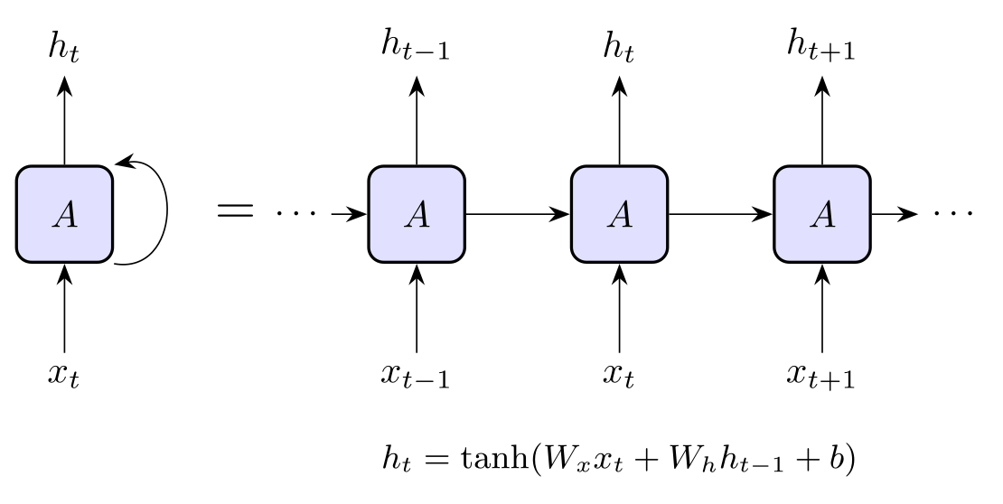
\usepackage{tikz} \usetikzlibrary{arrows.meta}\begin{tikzpicture}[>={Stealth[length=2mm]},
cell/.style={draw, thick, rounded corners, fill=blue!12, minimum size=9mm}]
% folded: the hidden state loops back into the cell
\node[cell] (A) at (0,0) {$A$};
\draw[->] (0,-1.3) node[below] {$x_t$} -- (A);
\draw[->] (A) -- (0,1.3) node[above] {$h_t$};
\draw[->] (A.south east) to[out=-10, in=10, looseness=1.8] (A.north east);
\node at (1.6,0) {\Large$=$};
% unrolled in time: one copy of the same cell per step
\foreach \t/\lab [count=\k] in {-1/{t-1}, 0/t, 1/{t+1}} {
\node[cell] (U\k) at ({5.2+1.9*\t},0) {$A$};
\draw[->] ({5.2+1.9*\t},-1.3) node[below] {$x_{\lab}$} -- (U\k);
\draw[->] (U\k) -- ({5.2+1.9*\t},1.3) node[above] {$h_{\lab}$};
}
\draw[->] (2.5,0) node[left] {$\cdots$} -- (U1);
\draw[->] (U1) -- (U2);
\draw[->] (U2) -- (U3);
\draw[->] (U3) -- (8,0) node[right] {$\cdots$};
\node[font=\small] at (5.2,-2.3) {$h_t = \tanh(W_x x_t + W_h h_{t-1} + b)$};
\end{tikzpicture}Full document
\documentclass[border=4pt]{standalone}
\usepackage{tikz}
\usetikzlibrary{arrows.meta}
\begin{document}
\begin{tikzpicture}[>={Stealth[length=2mm]},
    cell/.style={draw, thick, rounded corners, fill=blue!12, minimum size=9mm}]
  % folded: the hidden state loops back into the cell
  \node[cell] (A) at (0,0) {$A$};
  \draw[->] (0,-1.3) node[below] {$x_t$} -- (A);
  \draw[->] (A) -- (0,1.3) node[above] {$h_t$};
  \draw[->] (A.south east) to[out=-10, in=10, looseness=1.8] (A.north east);
  \node at (1.6,0) {\Large$=$};
  % unrolled in time: one copy of the same cell per step
  \foreach \t/\lab [count=\k] in {-1/{t-1}, 0/t, 1/{t+1}} {
    \node[cell] (U\k) at ({5.2+1.9*\t},0) {$A$};
    \draw[->] ({5.2+1.9*\t},-1.3) node[below] {$x_{\lab}$} -- (U\k);
    \draw[->] (U\k) -- ({5.2+1.9*\t},1.3) node[above] {$h_{\lab}$};
  }
  \draw[->] (2.5,0) node[left] {$\cdots$} -- (U1);
  \draw[->] (U1) -- (U2);
  \draw[->] (U2) -- (U3);
  \draw[->] (U3) -- (8,0) node[right] {$\cdots$};
  \node[font=\small] at (5.2,-2.3) {$h_t = \tanh(W_x x_t + W_h h_{t-1} + b)$};
\end{tikzpicture}
\end{document}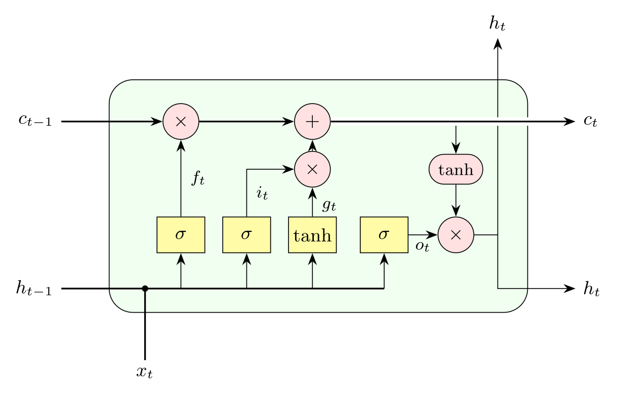
\usepackage{tikz} \usetikzlibrary{arrows.meta}\begin{tikzpicture}[>={Stealth[length=2mm]}, font=\small,
layer/.style={draw, fill=yellow!35, minimum width=8mm, minimum height=6mm, inner sep=1pt},
op/.style={circle, draw, fill=red!12, minimum size=6mm, inner sep=0pt},
lab/.style={font=\footnotesize, right=1pt}]
\draw[rounded corners=4mm, fill=green!6] (0,0) rectangle (7,3.9);
% gate layers (sigma = logistic sigmoid) and pointwise operations
\node[layer] (f) at (1.2,1.3) {$\sigma$};
\node[layer] (i) at (2.3,1.3) {$\sigma$};
\node[layer] (g) at (3.4,1.3) {$\tanh$};
\node[layer] (o) at (4.6,1.3) {$\sigma$};
\node[op] (mf) at (1.2,3.2) {$\times$};
\node[op] (pl) at (3.4,3.2) {$+$};
\node[op] (mi) at (3.4,2.4) {$\times$};
\node[op, rectangle, rounded corners=2.5mm, minimum width=9mm, minimum height=5mm] (tc) at (5.8,2.4) {\footnotesize$\tanh$};
\node[op] (mo) at (5.8,1.3) {$\times$};
% h_{t-1} and x_t are joined and feed all four layers
\draw[thick] (-0.8,0.4) node[left] {$h_{t-1}$} -- (4.6,0.4);
\draw[thick] (0.6,-0.8) node[below] {$x_t$} -- (0.6,0.4);
\fill (0.6,0.4) circle[radius=1.5pt];
\foreach \n in {f,i,g,o} \draw[->] (\n |- 0,0.4) -- (\n);
% gates acting on the cell state
\draw[->] (f) -- node[lab] {$f_t$} (mf);
\draw[->] (i) |- node[lab, pos=0.25] {$i_t$} (mi);
\draw[->] (g) -- node[lab, pos=0.35] {$g_t$} (mi);
\draw[->] (mi) -- (pl);
\draw[->] (o) -- node[below, font=\footnotesize] {$o_t$} (mo);
\draw[->] (5.8,3.2) -- (tc);
\draw[->] (tc) -- (mo);
% output h_t: to the next step and up out of the cell
\draw[->] (mo) -- (6.5,1.3) |- (7.8,0.4) node[right] {$h_t$};
\draw[->] (6.5,1.3) -- (6.5,4.6) node[above] {$h_t$};
% cell state along the top, drawn last with a white edge where h_t crosses it
\draw[->, thick] (-0.8,3.2) node[left] {$c_{t-1}$} -- (mf);
\draw[->, thick] (mf) -- (pl);
\draw[->, thick, preaction={draw, white, line width=4pt}] (pl) -- (7.8,3.2) node[right] {$c_t$};
\end{tikzpicture}Full document
\documentclass[border=4pt]{standalone}
\usepackage{tikz}
\usetikzlibrary{arrows.meta}
\begin{document}
\begin{tikzpicture}[>={Stealth[length=2mm]}, font=\small,
    layer/.style={draw, fill=yellow!35, minimum width=8mm, minimum height=6mm, inner sep=1pt},
    op/.style={circle, draw, fill=red!12, minimum size=6mm, inner sep=0pt},
    lab/.style={font=\footnotesize, right=1pt}]
  \draw[rounded corners=4mm, fill=green!6] (0,0) rectangle (7,3.9);
  % gate layers (sigma = logistic sigmoid) and pointwise operations
  \node[layer] (f) at (1.2,1.3) {$\sigma$};
  \node[layer] (i) at (2.3,1.3) {$\sigma$};
  \node[layer] (g) at (3.4,1.3) {$\tanh$};
  \node[layer] (o) at (4.6,1.3) {$\sigma$};
  \node[op] (mf) at (1.2,3.2) {$\times$};
  \node[op] (pl) at (3.4,3.2) {$+$};
  \node[op] (mi) at (3.4,2.4) {$\times$};
  \node[op, rectangle, rounded corners=2.5mm, minimum width=9mm, minimum height=5mm] (tc) at (5.8,2.4) {\footnotesize$\tanh$};
  \node[op] (mo) at (5.8,1.3) {$\times$};
  % h_{t-1} and x_t are joined and feed all four layers
  \draw[thick] (-0.8,0.4) node[left] {$h_{t-1}$} -- (4.6,0.4);
  \draw[thick] (0.6,-0.8) node[below] {$x_t$} -- (0.6,0.4);
  \fill (0.6,0.4) circle[radius=1.5pt];
  \foreach \n in {f,i,g,o} \draw[->] (\n |- 0,0.4) -- (\n);
  % gates acting on the cell state
  \draw[->] (f) -- node[lab] {$f_t$} (mf);
  \draw[->] (i) |- node[lab, pos=0.25] {$i_t$} (mi);
  \draw[->] (g) -- node[lab, pos=0.35] {$g_t$} (mi);
  \draw[->] (mi) -- (pl);
  \draw[->] (o) -- node[below, font=\footnotesize] {$o_t$} (mo);
  \draw[->] (5.8,3.2) -- (tc);
  \draw[->] (tc) -- (mo);
  % output h_t: to the next step and up out of the cell
  \draw[->] (mo) -- (6.5,1.3) |- (7.8,0.4) node[right] {$h_t$};
  \draw[->] (6.5,1.3) -- (6.5,4.6) node[above] {$h_t$};
  % cell state along the top, drawn last with a white edge where h_t crosses it
  \draw[->, thick] (-0.8,3.2) node[left] {$c_{t-1}$} -- (mf);
  \draw[->, thick] (mf) -- (pl);
  \draw[->, thick, preaction={draw, white, line width=4pt}] (pl) -- (7.8,3.2) node[right] {$c_t$};
\end{tikzpicture}
\end{document}Encoder–decoder and autoencoder
An autoencoder is a network whose layers narrow to a small code z and widen again to a reconstruction x̂ of the input, so it is the fully connected loop from the top of the page with the list {6,4,2,4,6}. The braces under the encoder and decoder halves come from the decorations.pathreplacing library: decoration={brace, mirror, amplitude=6pt}, where mirror turns the brace to point down and amplitude sets its height. The same arrangement serves for other encoder–decoder models; for a sequence-to-sequence model, chain two unrolled RNNs from the previous section, with the encoder’s last hidden state passed to the decoder.
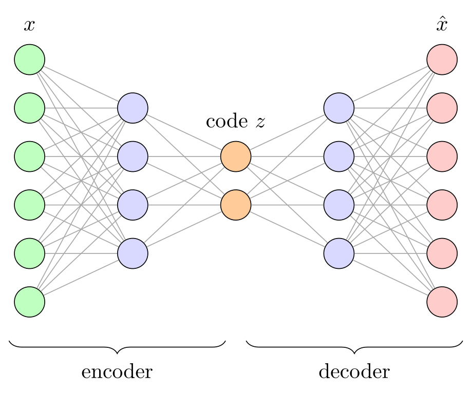
\usepackage{tikz} \usetikzlibrary{decorations.pathreplacing}\begin{tikzpicture}[x=1.7cm, y=0.8cm,
neuron/.style={circle, draw, minimum size=5mm, inner sep=0pt}]
% the same loop as for a plain network, with a narrow middle layer
\foreach \n/\c [count=\l, remember=\n as \prev (initially 0)] in
{6/green!25, 4/blue!15, 2/orange!40, 4/blue!15, 6/red!20} {
\foreach \i in {1,...,\n}
\node[neuron, fill=\c] (N\l-\i) at (\l, {(\n+1)/2 - \i}) {};
\ifnum\l>1
\pgfmathtruncatemacro\k{\l - 1}
\foreach \i in {1,...,\prev}
\foreach \j in {1,...,\n}
\draw[gray!70] (N\k-\i) -- (N\l-\j);
\fi
}
\node[above=1mm] at (N1-1.north) {$x$};
\node[above=1mm] at (N3-1.north) {code $z$};
\node[above=1mm] at (N5-1.north) {$\hat x$};
\draw[decorate, decoration={brace, mirror, amplitude=6pt}]
(0.8,-3.3) -- node[below=7pt] {encoder} (2.9,-3.3);
\draw[decorate, decoration={brace, mirror, amplitude=6pt}]
(3.1,-3.3) -- node[below=7pt] {decoder} (5.2,-3.3);
\end{tikzpicture}Full document
\documentclass[border=4pt]{standalone}
\usepackage{tikz}
\usetikzlibrary{decorations.pathreplacing}
\begin{document}
\begin{tikzpicture}[x=1.7cm, y=0.8cm,
    neuron/.style={circle, draw, minimum size=5mm, inner sep=0pt}]
  % the same loop as for a plain network, with a narrow middle layer
  \foreach \n/\c [count=\l, remember=\n as \prev (initially 0)] in
      {6/green!25, 4/blue!15, 2/orange!40, 4/blue!15, 6/red!20} {
    \foreach \i in {1,...,\n}
      \node[neuron, fill=\c] (N\l-\i) at (\l, {(\n+1)/2 - \i}) {};
    \ifnum\l>1
      \pgfmathtruncatemacro\k{\l - 1}
      \foreach \i in {1,...,\prev}
        \foreach \j in {1,...,\n}
          \draw[gray!70] (N\k-\i) -- (N\l-\j);
    \fi
  }
  \node[above=1mm] at (N1-1.north) {$x$};
  \node[above=1mm] at (N3-1.north) {code $z$};
  \node[above=1mm] at (N5-1.north) {$\hat x$};
  \draw[decorate, decoration={brace, mirror, amplitude=6pt}]
    (0.8,-3.3) -- node[below=7pt] {encoder} (2.9,-3.3);
  \draw[decorate, decoration={brace, mirror, amplitude=6pt}]
    (3.1,-3.3) -- node[below=7pt] {decoder} (5.2,-3.3);
\end{tikzpicture}
\end{document}Attention and the transformer block
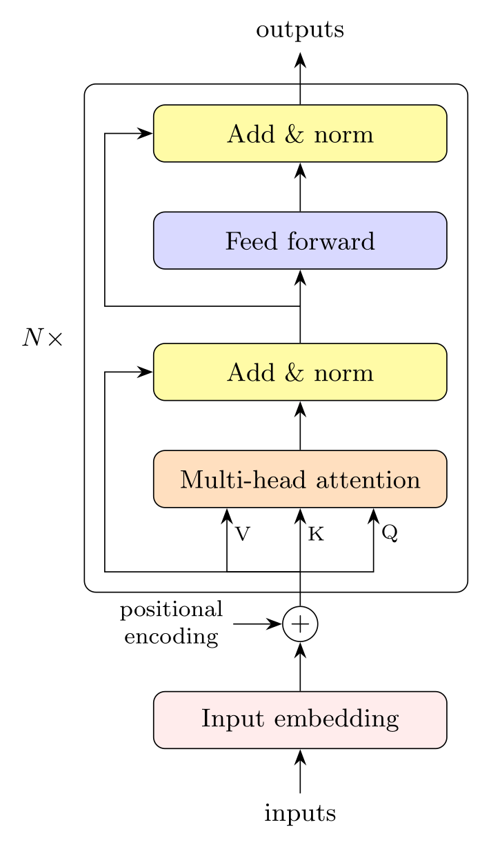
A transformer block is a flowchart: boxes placed with above=of from the positioning library, arrows between them, and residual connections routed around the side with |-. The picture is one encoder layer of the original transformer (Vaswani et al., 2017): multi-head self-attention, whose queries, keys and values (Q, K, V) all come from the same input, then “add & norm” (the residual sum followed by layer normalisation), a position-wise feed-forward network and a second add & norm. The fit library draws the frame around the layer, fit=(r1)(mha)(an2)(r2), and the N× beside it says that the layer is stacked; the paper uses N = 6, model width 512 and 8 attention heads.
Inside the attention box, each head computes Attention(Q, K, V) = softmax(QKT/√dk) V. Variants are small edits: many current models put the normalisation before each sub-layer (pre-norm), so the “norm” box moves below the attention and feed-forward boxes, and decoder-only models such as GPT use masked self-attention; the decoder of the original model adds a second, cross-attention sub-layer whose keys and values come from the encoder.
\usepackage{tikz} \usetikzlibrary{arrows.meta, positioning, fit, calc}\begin{tikzpicture}[>={Stealth[length=2mm]}, font=\small, node distance=6mm,
box/.style={draw, rounded corners, minimum width=3.6cm, minimum height=7mm, fill=#1},
box/.default=white]
% one encoder layer of the original transformer (post-norm)
\node[box=pink!30] (emb) {Input embedding};
\node[circle, draw, inner sep=1pt, above=of emb] (pe) {$+$};
\node[box=orange!25, above=12mm of pe] (mha) {Multi-head attention};
\node[box=yellow!35, above=of mha] (an1) {Add \& norm};
\node[box=blue!15, above=9mm of an1] (ff) {Feed forward};
\node[box=yellow!35, above=of ff] (an2) {Add \& norm};
\draw[<-] (emb) -- ++(0,-0.9) node[below] {inputs};
\draw[->] (emb) -- (pe);
\node[left=6mm of pe, align=center, font=\footnotesize] (pos) {positional\\encoding};
\draw[->] (pos) -- (pe);
% queries, keys and values all come from the same input (self-attention)
\coordinate (s1) at ($(pe)!0.45!(mha.south)$);
\draw (pe) -- (s1);
\foreach \dx/\q in {-9mm/V, 0mm/K, 9mm/Q}
\draw[->] (s1) -| node[pos=0.8, right=-1pt, font=\scriptsize] {\q} ([xshift=\dx]mha.south);
\draw[->] (mha) -- (an1);
\draw[->] (an1) -- (ff);
\draw[->] (ff) -- (an2);
\draw[->] (an2) -- ++(0,1) node[above] {outputs};
% residual connections around both sub-layers
\coordinate (s2) at ($(an1.north)!0.5!(ff.south)$);
\draw[->] (s1) -- ++(-2.4,0) coordinate (r1) |- (an1.west);
\draw[->] (s2) -- ++(-2.4,0) coordinate (r2) |- (an2.west);
\node[draw, rounded corners, fit=(r1)(mha)(an2)(r2), inner sep=2.5mm] (layer) {};
\node[left=1mm of layer] {$N\times$};
\end{tikzpicture}Full document
\documentclass[border=4pt]{standalone}
\usepackage{tikz}
\usetikzlibrary{arrows.meta, positioning, fit, calc}
\begin{document}
\begin{tikzpicture}[>={Stealth[length=2mm]}, font=\small, node distance=6mm,
    box/.style={draw, rounded corners, minimum width=3.6cm, minimum height=7mm, fill=#1},
    box/.default=white]
  % one encoder layer of the original transformer (post-norm)
  \node[box=pink!30]             (emb) {Input embedding};
  \node[circle, draw, inner sep=1pt, above=of emb] (pe) {$+$};
  \node[box=orange!25, above=12mm of pe] (mha) {Multi-head attention};
  \node[box=yellow!35, above=of mha]     (an1) {Add \& norm};
  \node[box=blue!15, above=9mm of an1]   (ff)  {Feed forward};
  \node[box=yellow!35, above=of ff]      (an2) {Add \& norm};
  \draw[<-] (emb) -- ++(0,-0.9) node[below] {inputs};
  \draw[->] (emb) -- (pe);
  \node[left=6mm of pe, align=center, font=\footnotesize] (pos) {positional\\encoding};
  \draw[->] (pos) -- (pe);
  % queries, keys and values all come from the same input (self-attention)
  \coordinate (s1) at ($(pe)!0.45!(mha.south)$);
  \draw (pe) -- (s1);
  \foreach \dx/\q in {-9mm/V, 0mm/K, 9mm/Q}
    \draw[->] (s1) -| node[pos=0.8, right=-1pt, font=\scriptsize] {\q} ([xshift=\dx]mha.south);
  \draw[->] (mha) -- (an1);
  \draw[->] (an1) -- (ff);
  \draw[->] (ff) -- (an2);
  \draw[->] (an2) -- ++(0,1) node[above] {outputs};
  % residual connections around both sub-layers
  \coordinate (s2) at ($(an1.north)!0.5!(ff.south)$);
  \draw[->] (s1) -- ++(-2.4,0) coordinate (r1) |- (an1.west);
  \draw[->] (s2) -- ++(-2.4,0) coordinate (r2) |- (an2.west);
  \node[draw, rounded corners, fit=(r1)(mha)(an2)(r2), inner sep=2.5mm] (layer) {};
  \node[left=1mm of layer] {$N\times$};
\end{tikzpicture}
\end{document}PlotNeuralNet and ready-made figures
PlotNeuralNet is a popular alternative for CNN figures in the 3D-box style (about 25,000 stars on GitHub, MIT licence). You describe the architecture in Python as a list of calls such as to_Conv, to_Pool, to_SoftMax, to_connection and to_skip, and to_generate writes a .tex file of TikZ code, which the repository’s tikzmake.sh script compiles. The generated file is not self-contained: it loads the repository’s layers/ folder with \subimport (and the TikZ positioning and 3d libraries), so keep that folder next to it or copy its style files. The last commit is from November 2020; the repository is not archived, but it is no longer developed.
The LabCanvas TikZ library has a whole category of machine learning examples: over fifty figures from open collections, each with its own MIT or CC0 licence and source, including neural network templates, VGG-16 and ResNet blocks, LSTM and GRU cells, attention and transformer diagrams and GANs. Every one opens in the TikZ editor, as does every snippet on this page.
Making the figures consistent
- Define the styles once (
neuron,layer,box) with\tikzsetin the preamble, so that every figure of a paper uses the same shapes and colours. - Space layers with
x=…andy=…on the picture rather than by changing coordinates; text keeps its size.scale=0.8also keeps text size, andtransform shapeshrinks the text with the drawing. - Use
font=\smallor\footnotesizefor labels on dense diagrams, and keep colour meaningful (inputs, hidden, outputs) rather than decorative. - When the figure must fit a fixed width, adjust the spacing until its natural size fits:
\resizeboxscales the text with the drawing, so the labels no longer match the font size of the document.
Common errors and how to fix them
| LaTeX says (or you see) | Cause and fix |
|---|---|
| Package pgf Error: No shape named `N0-1' is known. | The loop connects the first layer to a layer 0 that does not exist. Wrap the connections in \ifnum\l>1 … \fi. (Note that {1,...,0} counts down, 1 then 0, so an empty previous layer is not skipped by itself.) |
| Package pgfkeys Error: I do not know the key '/tikz/fit', to which you passed '(a)(b)', and I am going to ignore it. Perhaps you misspelled it. | A frame drawn with fit=… needs \usetikzlibrary{fit}. |
| Package PGF Math Error: Unknown function `of' (in 'of a'). | above=of a needs \usetikzlibrary{positioning}; without it, above= expects a distance. |
| Package pgfkeys Error: I do not know the key '/tikz/ellipse' and I am going to ignore it. Perhaps you misspelled it. | The ellipse node shape (also trapezium, diamond) is in \usetikzlibrary{shapes.geometric}; or use a rectangle with rounded corners. |
| Missing $ inserted. | A label such as {w_1} or {h_{t-1}} uses a subscript outside maths. Write {$w_1$}. |
| Package tikz Error: You need to load a decoration library. | The brace decoration needs \usetikzlibrary{decorations.pathreplacing}. |
Frequently asked questions
How do I draw a neural network in LaTeX?
With TikZ: place the neurons as circle nodes in nested \foreach loops (one over the layers, one over the neurons of a layer), name them by layer and index, and draw lines between all pairs of consecutive layers. The quick answer on this page draws a whole network from the list of layer sizes {3,5,5,2}.
How do I change the number of neurons or layers?
Edit the list in the \foreach: each entry is one layer, size/colour/label. The neurons are centred automatically with y = (n+1)/2 − i, and the connections follow the list, so no other line changes.
How do I draw a CNN diagram in LaTeX?
Draw each feature map as a pseudo-3D box (a front rectangle plus a top and a side parallelogram) defined once as a pic with arguments for thickness, height, depth and colour, and place the boxes in a row with arrows. PlotNeuralNet generates such figures from Python, but its output depends on the files in its repository.
How do I draw a transformer architecture in TikZ?
Treat it as a flowchart: boxes for embedding, multi-head attention, add & norm and feed forward placed with above=of (positioning library), arrows between them, residual connections routed with |-, and a frame from the fit library labelled N× for the stacked layers.
What is PlotNeuralNet?
A Python project (MIT licence) that writes TikZ code for neural network figures in a 3D-box style from a list of layer calls such as to_Conv and to_Pool. It needs its layers/ folder to compile and has not been updated since 2020.
How do I put labels on the edges of a neural network?
Add a node to the edge: \draw (a) -- node[pos=0.3, above, sloped] {$w_{11}$} (b);. sloped turns the label along the line, pos moves it along, and above or below picks the side. On crossing edges put the labels near the start and on the side facing empty space.
References
- PGF/TikZ manual, §88 Repeating Things: The Foreach Statement (count, remember)tikz.dev
- PGF/TikZ manual, §17.5.3 Advanced Placement Options (positioning)tikz.dev
- PGF/TikZ manual, §17.8 Placing Nodes on a Line or Curve Explicitly (pos, sloped)tikz.dev
- PGF/TikZ manual, §18.3 Defining New Pic Typestikz.dev
- PGF/TikZ manual, §87.4.4 Defining Styles (/.style n args)tikz.dev
- PGF/TikZ manual, §54 Fitting Librarytikz.dev
- PGF/TikZ manual, §50.4 Path Replacing Decorations (brace)tikz.dev
- PGF/TikZ manual, §24.4.1 Positioning Decorations Relative to the Path (mirror, raise)tikz.dev
- PGF/TikZ manual, §13.3.1 Intersections of Perpendicular Lines (|- and -|)tikz.dev
- PGF/TikZ manual, §15.10 Doing Multiple Actions on a Path (preaction)tikz.dev
- Vaswani et al., Attention Is All You Need (2017), arXiv:1706.03762arxiv.org
- PyTorch documentation: torch.nn.LSTM (gate equations)docs.pytorch.org
- PlotNeuralNet on GitHub (MIT licence)github.com
The facts on this page were checked against these sources, and every picture is the code with it typeset with TeX Live 2026. Code on this page: CC0 1.0, copy it freely.
Try the code in your browserEvery snippet on this page opens in the free TikZ editor: it is typeset with TeX Live as you type, with errors pointed at their line.
Open the TikZ editor