Bloch sphere in TikZ: drawing a qubit state in LaTeX
Quick answer
\shade[ball color=blue!15] (0,0) circle[radius=2];, draw the equator as an ellipse whose back (upper) half is dashed, and put the axes and the state vector on top. For a picture that is geometrically right, treat it as an orthographic view: seen from 20° above the equator, the equator is an ellipse 2 by 2 sin 20° cm, the pole sits at 2 cos 20° cm, and a point of the equator at azimuth φ is the elliptical polar coordinate ({250+φ}:{2} and {0.684}). The state θ, φ then lands at sin θ times that point plus cos θ times the pole, which calc computes. The convention is |ψ⟩ = cos(θ/2)|0⟩ + eiφ sin(θ/2)|1⟩, with |0⟩ at the top. The complete picture below takes the two angles as parameters.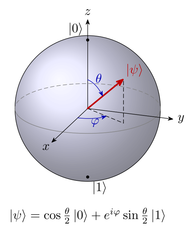
\usepackage{tikz} \usetikzlibrary{calc, arrows.meta}\begin{tikzpicture}[line cap=round, >={Stealth[round]}]
\def\Rs{2} % radius of the sphere (cm)
\def\El{20} % the view is 20 degrees above the equator
\def\Th{50} % polar angle theta of the state
\def\Ph{60} % azimuth phi of the state
\pgfmathsetmacro\Ry{\Rs*sin(\El)} % half-height of the equator ellipse
\pgfmathsetmacro\Zh{\Rs*cos(\El)} % height of the north pole
% sphere, then the equator: back half dashed, front half solid
\shade[ball color=blue!15, opacity=0.7] (0,0) circle[radius=\Rs];
\draw (0,0) circle[radius=\Rs];
\draw[densely dashed, gray] (\Rs,0) arc[start angle=0, end angle=180, x radius=\Rs, y radius=\Ry];
\draw[gray] (-\Rs,0) arc[start angle=180, end angle=360, x radius=\Rs, y radius=\Ry];
% axes: x and y end on the equator, 90 degrees apart; z ends at the pole
\coordinate (O) at (0,0);
\coordinate (X) at (250:{\Rs} and {\Ry});
\coordinate (Y) at (340:{\Rs} and {\Ry});
\coordinate (Z) at (0,\Zh);
\draw[->] (O) -- ($1.45*(X)$) node[below left=-2pt] {$x$};
\draw[->] (O) -- ($1.25*(Y)$) node[right] {$y$};
\draw[->] (O) -- ($1.3*(Z)$) node[above] {$z$};
\fill (Z) circle[radius=1.2pt] node[above left] {$|0\rangle$};
\fill (0,-\Zh) circle[radius=1.2pt] node[below right] {$|1\rangle$};
% the state: P = sin(theta)*(equator point at phi) + cos(theta)*(pole)
\coordinate (F) at ($sin(\Th)*({250+\Ph}:{\Rs} and {\Ry})$);
\coordinate (P) at ($(F) + cos(\Th)*(Z)$);
\draw[densely dashed] (O) -- (F) -- (P);
\draw[->, very thick, red!75!black] (O) -- (P) node[above right=-2pt] {$|\psi\rangle$};
% phi: from the x axis to the foot F, in the equator plane
\draw[->, blue!70!black] (250:{0.4*\Rs} and {0.4*\Ry})
arc[start angle=250, delta angle=\Ph, x radius=0.4*\Rs, y radius=0.4*\Ry];
\node[blue!70!black] at ({250+\Ph/2}:{0.58*\Rs} and {0.58*\Ry}) {$\varphi$};
% theta: from the z axis down to the state, in the plane of z and P
\draw[->, blue!70!black] plot[domain=0:\Th, samples=25]
({0.42*sin(\x)*\Rs*cos(250+\Ph)}, {0.42*(sin(\x)*\Ry*sin(250+\Ph) + cos(\x)*\Zh)});
\node[blue!70!black] at ({0.56*sin(\Th/2)*\Rs*cos(250+\Ph)}, {0.56*(sin(\Th/2)*\Ry*sin(250+\Ph) + cos(\Th/2)*\Zh)}) {$\theta$};
\node[below=6mm, align=center] at (0,-\Rs)
{$|\psi\rangle = \cos\frac{\theta}{2}\,|0\rangle + e^{i\varphi}\sin\frac{\theta}{2}\,|1\rangle$};
\end{tikzpicture}Full document
\documentclass[border=4pt]{standalone}
\usepackage{tikz}
\usetikzlibrary{calc, arrows.meta}
\begin{document}
\begin{tikzpicture}[line cap=round, >={Stealth[round]}]
  \def\Rs{2}   % radius of the sphere (cm)
  \def\El{20}  % the view is 20 degrees above the equator
  \def\Th{50}  % polar angle theta of the state
  \def\Ph{60}  % azimuth phi of the state
  \pgfmathsetmacro\Ry{\Rs*sin(\El)}  % half-height of the equator ellipse
  \pgfmathsetmacro\Zh{\Rs*cos(\El)}  % height of the north pole
  % sphere, then the equator: back half dashed, front half solid
  \shade[ball color=blue!15, opacity=0.7] (0,0) circle[radius=\Rs];
  \draw (0,0) circle[radius=\Rs];
  \draw[densely dashed, gray] (\Rs,0) arc[start angle=0, end angle=180, x radius=\Rs, y radius=\Ry];
  \draw[gray] (-\Rs,0) arc[start angle=180, end angle=360, x radius=\Rs, y radius=\Ry];
  % axes: x and y end on the equator, 90 degrees apart; z ends at the pole
  \coordinate (O) at (0,0);
  \coordinate (X) at (250:{\Rs} and {\Ry});
  \coordinate (Y) at (340:{\Rs} and {\Ry});
  \coordinate (Z) at (0,\Zh);
  \draw[->] (O) -- ($1.45*(X)$) node[below left=-2pt] {$x$};
  \draw[->] (O) -- ($1.25*(Y)$) node[right] {$y$};
  \draw[->] (O) -- ($1.3*(Z)$) node[above] {$z$};
  \fill (Z) circle[radius=1.2pt] node[above left] {$|0\rangle$};
  \fill (0,-\Zh) circle[radius=1.2pt] node[below right] {$|1\rangle$};
  % the state: P = sin(theta)*(equator point at phi) + cos(theta)*(pole)
  \coordinate (F) at ($sin(\Th)*({250+\Ph}:{\Rs} and {\Ry})$);
  \coordinate (P) at ($(F) + cos(\Th)*(Z)$);
  \draw[densely dashed] (O) -- (F) -- (P);
  \draw[->, very thick, red!75!black] (O) -- (P) node[above right=-2pt] {$|\psi\rangle$};
  % phi: from the x axis to the foot F, in the equator plane
  \draw[->, blue!70!black] (250:{0.4*\Rs} and {0.4*\Ry})
    arc[start angle=250, delta angle=\Ph, x radius=0.4*\Rs, y radius=0.4*\Ry];
  \node[blue!70!black] at ({250+\Ph/2}:{0.58*\Rs} and {0.58*\Ry}) {$\varphi$};
  % theta: from the z axis down to the state, in the plane of z and P
  \draw[->, blue!70!black] plot[domain=0:\Th, samples=25]
    ({0.42*sin(\x)*\Rs*cos(250+\Ph)}, {0.42*(sin(\x)*\Ry*sin(250+\Ph) + cos(\x)*\Zh)});
  \node[blue!70!black] at ({0.56*sin(\Th/2)*\Rs*cos(250+\Ph)}, {0.56*(sin(\Th/2)*\Ry*sin(250+\Ph) + cos(\Th/2)*\Zh)}) {$\theta$};
  \node[below=6mm, align=center] at (0,-\Rs)
    {$|\psi\rangle = \cos\frac{\theta}{2}\,|0\rangle + e^{i\varphi}\sin\frac{\theta}{2}\,|1\rangle$};
\end{tikzpicture}
\end{document}Contents
The state, the angles and the six basis states
A pure qubit state can be written, up to a global phase that has no physical meaning, as
|ψ⟩ = cos(θ/2) |0⟩ + eiφ sin(θ/2) |1⟩, 0 ≤ θ ≤ π, 0 ≤ φ < 2π,
and drawn as the point of the unit sphere with polar angle θ (from the +z axis) and azimuth φ (from +x towards +y): the Bloch vector (sin θ cos φ, sin θ sin φ, cos θ). Because the state uses θ/2, orthogonal states are antipodal: |0⟩ at the north pole and |1⟩ at the south pole are 180° apart on the sphere although they are 90° apart as vectors. Mixed states are the points inside the ball: ρ = ½(I + a·σ) with |a| ≤ 1, pure states on the surface.
| State | θ, φ | Bloch vector | Axis |
|---|---|---|---|
| |0⟩ | 0, any | (0, 0, 1) | +z (top) |
| |1⟩ | π, any | (0, 0, −1) | −z (bottom) |
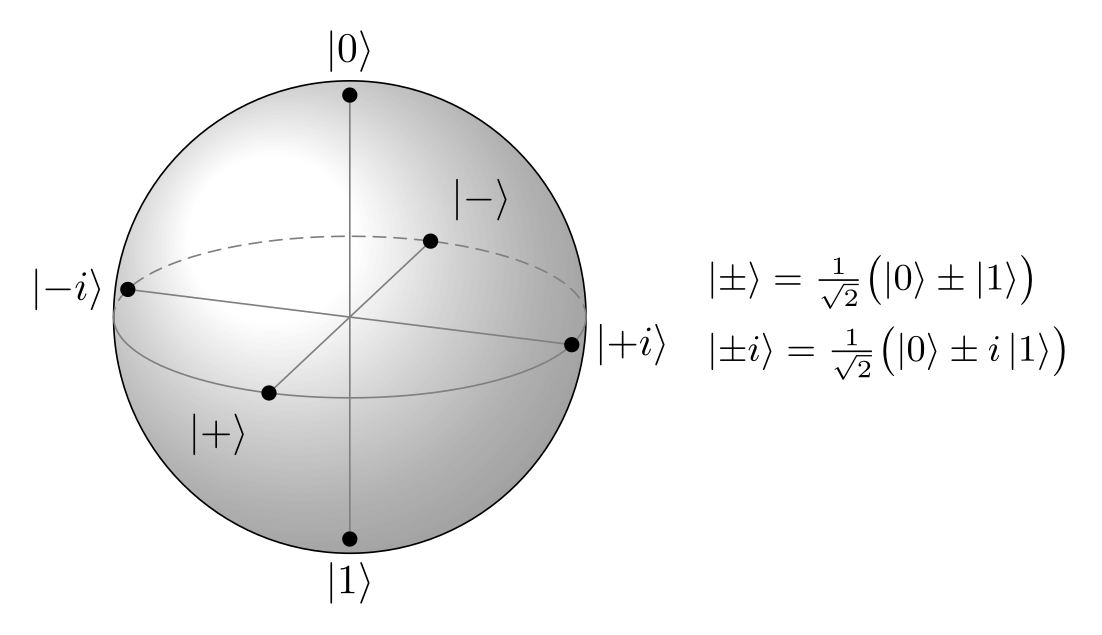
| |+⟩ = (|0⟩ + |1⟩)/√2 | π/2, 0 | (1, 0, 0) | +x |
| |−⟩ = (|0⟩ − |1⟩)/√2 | π/2, π | (−1, 0, 0) | −x |
| |+i⟩ = (|0⟩ + i|1⟩)/√2 | π/2, π/2 | (0, 1, 0) | +y |
| |−i⟩ = (|0⟩ − i|1⟩)/√2 | π/2, 3π/2 | (0, −1, 0) | −y |
The picture below puts the six states where the axes meet the sphere. In the code, $|{+}\rangle$ has braces around the sign: without them TeX treats + and − as binary operators and adds space around them.
\usepackage{tikz} \usetikzlibrary{calc}\begin{tikzpicture}[line cap=round, dot/.style={circle, fill, inner sep=1.3pt}]
\def\Rs{2}
\def\El{20}
\pgfmathsetmacro\Ry{\Rs*sin(\El)}
\pgfmathsetmacro\Zh{\Rs*cos(\El)}
\shade[ball color=white, opacity=0.6] (0,0) circle[radius=\Rs];
\draw (0,0) circle[radius=\Rs];
\draw[densely dashed, gray] (\Rs,0) arc[start angle=0, end angle=180, x radius=\Rs, y radius=\Ry];
\draw[gray] (-\Rs,0) arc[start angle=180, end angle=360, x radius=\Rs, y radius=\Ry];
% the six states where the axes meet the sphere
\coordinate (X) at (250:{\Rs} and {\Ry});
\coordinate (Y) at (340:{\Rs} and {\Ry});
\coordinate (Z) at (0,\Zh);
\draw[gray] ($-1*(X)$) -- (X) ($-1*(Y)$) -- (Y) (0,-\Zh) -- (Z);
\node[dot, label=above:{$|0\rangle$}] at (Z) {};
\node[dot, label=below:{$|1\rangle$}] at (0,-\Zh) {};
\node[dot, label=below left:{$|{+}\rangle$}] at (X) {};
\node[dot, label=above right:{$|{-}\rangle$}] at ($-1*(X)$) {};
\node[dot, label=right:{$|{+}i\rangle$}] at (Y) {};
\node[dot, label=left:{$|{-}i\rangle$}] at ($-1*(Y)$) {};
% what they are
\node[right, font=\small, align=left] at (2.9,0) {%
$|{\pm}\rangle = \frac{1}{\sqrt2}\bigl(|0\rangle \pm |1\rangle\bigr)$\\[3pt]
$|{\pm}i\rangle = \frac{1}{\sqrt2}\bigl(|0\rangle \pm i\,|1\rangle\bigr)$};
\end{tikzpicture}Full document
\documentclass[border=4pt]{standalone}
\usepackage{tikz}
\usetikzlibrary{calc}
\begin{document}
\begin{tikzpicture}[line cap=round, dot/.style={circle, fill, inner sep=1.3pt}]
  \def\Rs{2}
  \def\El{20}
  \pgfmathsetmacro\Ry{\Rs*sin(\El)}
  \pgfmathsetmacro\Zh{\Rs*cos(\El)}
  \shade[ball color=white, opacity=0.6] (0,0) circle[radius=\Rs];
  \draw (0,0) circle[radius=\Rs];
  \draw[densely dashed, gray] (\Rs,0) arc[start angle=0, end angle=180, x radius=\Rs, y radius=\Ry];
  \draw[gray] (-\Rs,0) arc[start angle=180, end angle=360, x radius=\Rs, y radius=\Ry];
  % the six states where the axes meet the sphere
  \coordinate (X) at (250:{\Rs} and {\Ry});
  \coordinate (Y) at (340:{\Rs} and {\Ry});
  \coordinate (Z) at (0,\Zh);
  \draw[gray] ($-1*(X)$) -- (X)  ($-1*(Y)$) -- (Y)  (0,-\Zh) -- (Z);
  \node[dot, label=above:{$|0\rangle$}]             at (Z) {};
  \node[dot, label=below:{$|1\rangle$}]             at (0,-\Zh) {};
  \node[dot, label=below left:{$|{+}\rangle$}]      at (X) {};
  \node[dot, label=above right:{$|{-}\rangle$}]     at ($-1*(X)$) {};
  \node[dot, label=right:{$|{+}i\rangle$}]          at (Y) {};
  \node[dot, label=left:{$|{-}i\rangle$}]           at ($-1*(Y)$) {};
  % what they are
  \node[right, font=\small, align=left] at (2.9,0) {%
    $|{\pm}\rangle = \frac{1}{\sqrt2}\bigl(|0\rangle \pm |1\rangle\bigr)$\\[3pt]
    $|{\pm}i\rangle = \frac{1}{\sqrt2}\bigl(|0\rangle \pm i\,|1\rangle\bigr)$};
\end{tikzpicture}
\end{document}Drawing the sphere: shading, outline and equator
A Bloch sphere is a 3D object, but plain TikZ draws in 2D, so decide on a view and project. The cleanest is an orthographic view from a little above the equator (20° in the code on this page):
- the outline is a circle of radius R, whatever the view, so it can be shaded with
ball color; theballshading is always defined, no library needed, andopacity=0.7lets the axes show through; - the equator is an ellipse with half-axes R and R sin 20°; seen from above, its far half is the upper half, so that half is dashed:
arc[start angle=0, end angle=180, x radius=\Rs, y radius=\Ry]; - the north pole is at height R cos 20°, a little below the top of the outline. Putting |0⟩ exactly on the outline, as many sketches do, is a different (inconsistent) projection;
- a point of the equator is an elliptical polar coordinate,
(angle:{x radius} and {y radius}). Looking from 20° round from the x axis, +x ends at the angle 250° of the ellipse and +y at 340°, and in general azimuth φ is at 250° + φ. To turn the view by some angle, subtract it from both numbers.
Write the radii in braces: TeX drops the space after a macro, so (250:\Rs and \Ry) reaches TikZ as 2and 0.68405 and stops with a maths error (see the errors below).
The state vector |ψ⟩ with θ and φ
With the equator points known, the state is a weighted sum, which the calc library evaluates: the foot of the vector in the equator plane is (F) = ($sin(\Th)*({250+\Ph}:{\Rs} and {\Ry})$), and the tip is (P) = ($(F) + cos(\Th)*(Z)$) with (Z) the pole. This is exact for every θ and φ, so the quick-answer code redraws itself when you change \Th and \Ph. The dashed path (O) -- (F) -- (P) shows the projection.
The angle marks follow the same idea. φ lies in the equator plane, so its mark is an elliptical arc with the same proportions as the equator, from 250° to 250° + φ. θ lies in the vertical plane through the state; its mark is a short plot of the points sin u · (equator point at φ) + cos u · (pole) for u from 0 to θ, scaled down. For a state on the far side of the sphere (with this view, roughly 110° < φ < 290° near the equator) draw the arrow dashed or lighter, as the equator’s back half.
Rotations: the state on a circle of latitude
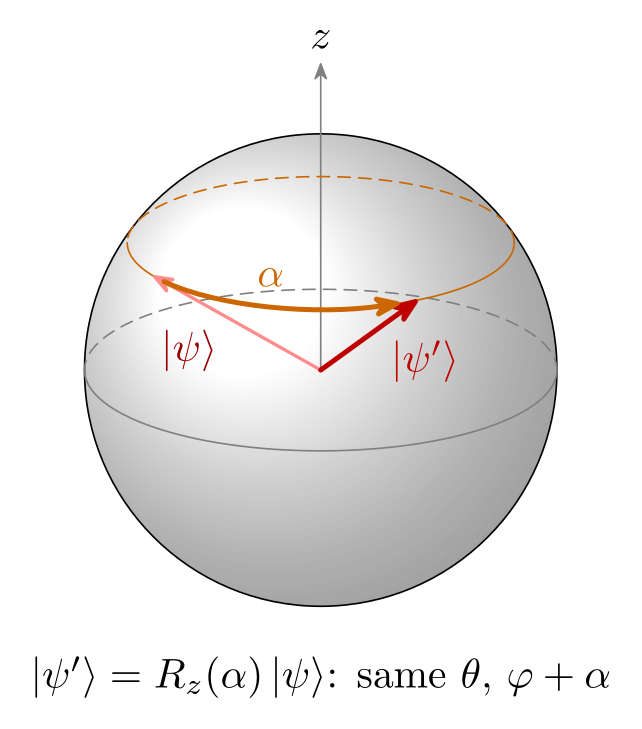
A rotation about z, Rz(α) = e−iαZ/2, keeps θ and adds α to φ (up to a global phase), so the state moves along the circle of latitude at θ; Larmor precession of a spin in a field along z looks the same. That circle is the equator shrunk by sin θ and lifted to the height R cos θ cos 20°, so it is drawn exactly like the equator: dashed upper half, solid lower half. The rotation arrow is an arc of the same ellipse between the two states.
\usepackage{tikz} \usetikzlibrary{calc, arrows.meta}\begin{tikzpicture}[line cap=round, >={Stealth[round]}]
\def\Rs{2}
\def\El{20}
\def\Th{55} % theta of the state (kept by R_z)
\def\PhA{-40} % phi before ...
\def\PhB{50} % ... and after R_z(90 degrees)
\pgfmathsetmacro\Ry{\Rs*sin(\El)}
\pgfmathsetmacro\Zh{\Rs*cos(\El)}
\pgfmathsetmacro\Cy{\Zh*cos(\Th)} % height of the circle of latitude
\pgfmathsetmacro\Ra{\Rs*sin(\Th)} % its radius ...
\pgfmathsetmacro\Rb{\Ry*sin(\Th)} % ... and half-height in the picture
\shade[ball color=white, opacity=0.6] (0,0) circle[radius=\Rs];
\draw (0,0) circle[radius=\Rs];
\draw[densely dashed, gray] (\Rs,0) arc[start angle=0, end angle=180, x radius=\Rs, y radius=\Ry];
\draw[gray] (-\Rs,0) arc[start angle=180, end angle=360, x radius=\Rs, y radius=\Ry];
\draw[->, gray] (0,0) -- (0,1.3*\Rs) node[above, black] {$z$};
% circle of latitude theta: centre (0,Cy), back half dashed
\coordinate (C) at (0,\Cy);
\draw[densely dashed, orange!80!black] ($(C)+(\Ra,0)$)
arc[start angle=0, end angle=180, x radius=\Ra, y radius=\Rb];
\draw[orange!80!black] ($(C)+(-\Ra,0)$)
arc[start angle=180, end angle=360, x radius=\Ra, y radius=\Rb];
% the state before and after the rotation, and the rotation along the circle
\coordinate (A) at ($(C)+({250+\PhA}:{\Ra} and {\Rb})$);
\coordinate (B) at ($(C)+({250+\PhB}:{\Ra} and {\Rb})$);
\draw[->, thick, red!45] (0,0) -- (A)
node[pos=0.55, below left=-1pt, red!60!black] {$|\psi\rangle$};
\draw[->, very thick, red!75!black] (0,0) -- (B)
node[pos=0.6, below right=-1pt] {$|\psi'\rangle$};
\draw[->, very thick, orange!80!black] ($(C)+({250+\PhA+6}:{\Ra} and {\Rb})$)
arc[start angle=250+\PhA+6, end angle=250+\PhB-6, x radius=\Ra, y radius=\Rb]
node[midway, above=1pt] {$\alpha$};
\node[below=3mm] at (0,-\Rs) {$|\psi'\rangle = R_z(\alpha)\,|\psi\rangle$: same $\theta$, $\varphi + \alpha$};
\end{tikzpicture}Full document
\documentclass[border=4pt]{standalone}
\usepackage{tikz}
\usetikzlibrary{calc, arrows.meta}
\begin{document}
\begin{tikzpicture}[line cap=round, >={Stealth[round]}]
  \def\Rs{2}
  \def\El{20}
  \def\Th{55}                     % theta of the state (kept by R_z)
  \def\PhA{-40}                   % phi before ...
  \def\PhB{50}                    % ... and after R_z(90 degrees)
  \pgfmathsetmacro\Ry{\Rs*sin(\El)}
  \pgfmathsetmacro\Zh{\Rs*cos(\El)}
  \pgfmathsetmacro\Cy{\Zh*cos(\Th)}  % height of the circle of latitude
  \pgfmathsetmacro\Ra{\Rs*sin(\Th)}  % its radius ...
  \pgfmathsetmacro\Rb{\Ry*sin(\Th)}  % ... and half-height in the picture
  \shade[ball color=white, opacity=0.6] (0,0) circle[radius=\Rs];
  \draw (0,0) circle[radius=\Rs];
  \draw[densely dashed, gray] (\Rs,0) arc[start angle=0, end angle=180, x radius=\Rs, y radius=\Ry];
  \draw[gray] (-\Rs,0) arc[start angle=180, end angle=360, x radius=\Rs, y radius=\Ry];
  \draw[->, gray] (0,0) -- (0,1.3*\Rs) node[above, black] {$z$};
  % circle of latitude theta: centre (0,Cy), back half dashed
  \coordinate (C) at (0,\Cy);
  \draw[densely dashed, orange!80!black] ($(C)+(\Ra,0)$)
    arc[start angle=0, end angle=180, x radius=\Ra, y radius=\Rb];
  \draw[orange!80!black] ($(C)+(-\Ra,0)$)
    arc[start angle=180, end angle=360, x radius=\Ra, y radius=\Rb];
  % the state before and after the rotation, and the rotation along the circle
  \coordinate (A) at ($(C)+({250+\PhA}:{\Ra} and {\Rb})$);
  \coordinate (B) at ($(C)+({250+\PhB}:{\Ra} and {\Rb})$);
  \draw[->, thick, red!45] (0,0) -- (A)
    node[pos=0.55, below left=-1pt, red!60!black] {$|\psi\rangle$};
  \draw[->, very thick, red!75!black] (0,0) -- (B)
    node[pos=0.6, below right=-1pt] {$|\psi'\rangle$};
  \draw[->, very thick, orange!80!black] ($(C)+({250+\PhA+6}:{\Ra} and {\Rb})$)
    arc[start angle=250+\PhA+6, end angle=250+\PhB-6, x radius=\Ra, y radius=\Rb]
    node[midway, above=1pt] {$\alpha$};
  \node[below=3mm] at (0,-\Rs) {$|\psi'\rangle = R_z(\alpha)\,|\psi\rangle$: same $\theta$, $\varphi + \alpha$};
\end{tikzpicture}
\end{document}The same sphere with tikz-3dplot
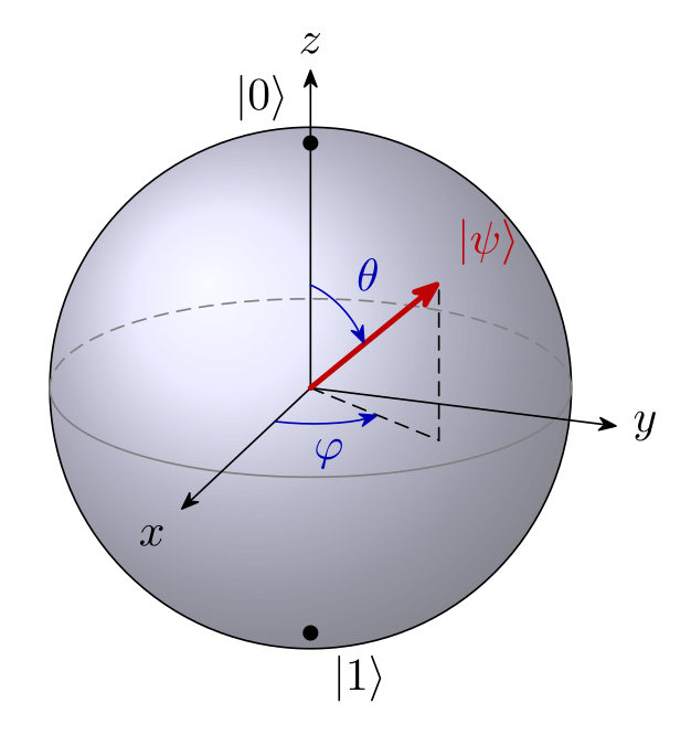
The tikz-3dplot package (version 2012-01-11, in TeX Live and MiKTeX) does the projection for you: \tdplotsetmaincoords{70}{110} rotates the frame by 70° about x and 110° about z, and the style tdplot_main_coords then lets you write 3D points such as (0,0,1). That view is the same as on the rest of this page (20° above the equator, 90° − 70°), and the picture comes out identical, because both are orthographic.
\tdplotsetcoord{P}{1}{\Th}{\Ph}defines the pointPfrom spherical coordinates (r, θ, φ) together with its projections, of which(Pxy)is the foot in the equator plane.\tdplotdrawarc[⟨style⟩]{⟨centre⟩}{⟨radius⟩}{⟨start⟩}{⟨end⟩}{⟨label options⟩}{⟨label⟩}draws an arc in the xy plane, with angles measured from x: the equator and the φ mark. After\tdplotsetthetaplanecoords{\Ph}, the same command withtdplot_rotated_coordsdraws in the vertical plane of the state, which gives the θ mark.- The outline is a circle on the page, not in 3D: draw it with
tdplot_screen_coords, or it comes out as a flat ellipse. - Which half of the equator faces you depends on the second angle: the half from φd − 180° to φd (here −70° to 110°) is in front.
\usepackage{tikz} \usepackage{tikz-3dplot} \usetikzlibrary{arrows.meta}\tdplotsetmaincoords{70}{110}%
\begin{tikzpicture}[scale=2, tdplot_main_coords, line cap=round, >={Stealth[round]}]
\def\Th{50}
\def\Ph{60}
% the outline is a circle on the page: draw it in screen coordinates
\shade[tdplot_screen_coords, ball color=blue!15, opacity=0.7] (0,0) circle[radius=1];
\draw[tdplot_screen_coords] (0,0) circle[radius=1];
% equator: azimuths -70 to 110 face the viewer (110 = the second angle above)
\tdplotdrawarc[gray]{(0,0,0)}{1}{-70}{110}{}{}
\tdplotdrawarc[gray, densely dashed]{(0,0,0)}{1}{110}{290}{}{}
\draw[->] (0,0,0) -- (1.45,0,0) node[anchor=north east] {$x$};
\draw[->] (0,0,0) -- (0,1.25,0) node[anchor=west] {$y$};
\draw[->] (0,0,0) -- (0,0,1.3) node[anchor=south] {$z$};
\node[circle, fill, inner sep=1.2pt, label=above left:{$|0\rangle$}] at (0,0,1) {};
\node[circle, fill, inner sep=1.2pt, label=below right:{$|1\rangle$}] at (0,0,-1) {};
% the state at (r, theta, phi); also defines (Pxy), its foot in the xy plane
\tdplotsetcoord{P}{1}{\Th}{\Ph}
\draw[densely dashed] (0,0,0) -- (Pxy) -- (P);
\draw[->, very thick, red!75!black] (0,0,0) -- (P) node[anchor=south west] {$|\psi\rangle$};
\tdplotdrawarc[->, blue!70!black]{(0,0,0)}{0.4}{0}{\Ph}{anchor=north}{$\varphi$}
\tdplotsetthetaplanecoords{\Ph}
\tdplotdrawarc[tdplot_rotated_coords, ->, blue!70!black]{(0,0,0)}{0.42}{0}{\Th}{anchor=south west}{$\theta$}
\end{tikzpicture}Full document
\documentclass[border=4pt]{standalone}
\usepackage{tikz}
\usepackage{tikz-3dplot}
\usetikzlibrary{arrows.meta}
\begin{document}
\tdplotsetmaincoords{70}{110}%
\begin{tikzpicture}[scale=2, tdplot_main_coords, line cap=round, >={Stealth[round]}]
  \def\Th{50}
  \def\Ph{60}
  % the outline is a circle on the page: draw it in screen coordinates
  \shade[tdplot_screen_coords, ball color=blue!15, opacity=0.7] (0,0) circle[radius=1];
  \draw[tdplot_screen_coords] (0,0) circle[radius=1];
  % equator: azimuths -70 to 110 face the viewer (110 = the second angle above)
  \tdplotdrawarc[gray]{(0,0,0)}{1}{-70}{110}{}{}
  \tdplotdrawarc[gray, densely dashed]{(0,0,0)}{1}{110}{290}{}{}
  \draw[->] (0,0,0) -- (1.45,0,0) node[anchor=north east] {$x$};
  \draw[->] (0,0,0) -- (0,1.25,0) node[anchor=west] {$y$};
  \draw[->] (0,0,0) -- (0,0,1.3) node[anchor=south] {$z$};
  \node[circle, fill, inner sep=1.2pt, label=above left:{$|0\rangle$}] at (0,0,1) {};
  \node[circle, fill, inner sep=1.2pt, label=below right:{$|1\rangle$}] at (0,0,-1) {};
  % the state at (r, theta, phi); also defines (Pxy), its foot in the xy plane
  \tdplotsetcoord{P}{1}{\Th}{\Ph}
  \draw[densely dashed] (0,0,0) -- (Pxy) -- (P);
  \draw[->, very thick, red!75!black] (0,0,0) -- (P) node[anchor=south west] {$|\psi\rangle$};
  \tdplotdrawarc[->, blue!70!black]{(0,0,0)}{0.4}{0}{\Ph}{anchor=north}{$\varphi$}
  \tdplotsetthetaplanecoords{\Ph}
  \tdplotdrawarc[tdplot_rotated_coords, ->, blue!70!black]{(0,0,0)}{0.42}{0}{\Th}{anchor=south west}{$\theta$}
\end{tikzpicture}
\end{document}The blochsphere package
There is a dedicated package on CTAN, blochsphere by Matthew Wardrop (version 1.1 of 2015-09-15, LPPL 1.3, in TeX Live and MiKTeX), and it compiles on TeX Live 2026. It provides a blochsphere environment with the options radius (default 1.5cm), tilt (15), rotation (−20), color, opacity (0.7) and nested=true for use inside a tikzpicture, and macros such as \drawBallGrid, \drawLatitudeCircle, \drawLongitudeCircle, \drawAxis, \labelPolar, \drawStatePolar{⟨name⟩}{⟨θ⟩}{⟨φ⟩} and \drawRotationLeft/Right; hidden parts are drawn faded automatically.
Things we found when rendering it, worth knowing before you use it:
- Its azimuth increases clockwise seen from above, so with z up its own axes form a left-handed frame. To get the usual picture (x towards you, y to the right), label its azimuth 90 as x and azimuth 0 as y, and draw a state (θ, φ) as
\drawStatePolar{psi}{θ}{90-φ}, as in the code below. - Keep
rotationnear its default: atrotation=-110the front half of the equator was drawn as hidden. - The poles are drawn at the top and bottom of the outline (the manual calls the drawing pseudo-3D), there is no command for angle marks, and the example in its manual puts |1⟩ at the top, the opposite of the quantum-computing convention.
The package has not been updated since 2015. For figures in a paper, the hand-built or tikz-3dplot versions give you full control with a few more lines.
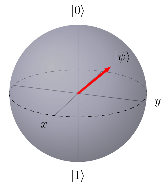
\usepackage{tikz} \usepackage{blochsphere}% blochsphere's azimuth runs clockwise seen from above, so Bloch x is its
% azimuth 90 and Bloch y its azimuth 0: draw a state (theta, phi) at {theta}{90-phi}
\begin{blochsphere}[radius=2cm, tilt=20, rotation=-20, color=blue!15, opacity=0.5]
\drawLatitudeCircle[style={dashed}]{0}
\drawAxis{0}{0}
\drawAxis{90}{90}
\drawAxis{90}{0}
\labelPolar[scale=1.15]{zp}{0}{0}
\labelPolar[scale=1.15]{zm}{180}{0}
\labelPolar[scale=1.2]{xp}{90}{90}
\labelPolar[scale=1.15]{yp}{90}{0}
\node[above] at (zp) {$|0\rangle$};
\node[below] at (zm) {$|1\rangle$};
\node[below left] at (xp) {$x$};
\node[right] at (yp) {$y$};
\drawStatePolar[statecolor=red, statewidth=1pt]{psi}{50}{30} % theta 50, phi 60
\node[above right] at (psi) {$|\psi\rangle$};
\end{blochsphere}Full document
\documentclass[border=4pt]{standalone}
\usepackage{tikz}
\usepackage{blochsphere}
\begin{document}
% blochsphere's azimuth runs clockwise seen from above, so Bloch x is its
% azimuth 90 and Bloch y its azimuth 0: draw a state (theta, phi) at {theta}{90-phi}
\begin{blochsphere}[radius=2cm, tilt=20, rotation=-20, color=blue!15, opacity=0.5]
  \drawLatitudeCircle[style={dashed}]{0}
  \drawAxis{0}{0}
  \drawAxis{90}{90}
  \drawAxis{90}{0}
  \labelPolar[scale=1.15]{zp}{0}{0}
  \labelPolar[scale=1.15]{zm}{180}{0}
  \labelPolar[scale=1.2]{xp}{90}{90}
  \labelPolar[scale=1.15]{yp}{90}{0}
  \node[above] at (zp) {$|0\rangle$};
  \node[below] at (zm) {$|1\rangle$};
  \node[below left] at (xp) {$x$};
  \node[right] at (yp) {$y$};
  \drawStatePolar[statecolor=red, statewidth=1pt]{psi}{50}{30}  % theta 50, phi 60
  \node[above right] at (psi) {$|\psi\rangle$};
\end{blochsphere}
\end{document}Quantum circuits and other figures
A Bloch sphere often sits next to a circuit: quantum circuits are drawn with the quantikz package. The TikZ physics examples include another Bloch sphere, from Janosh Riebesell’s diagrams collection, with its code. Every snippet on this page opens in the TikZ editor, where you can change \Th, \Ph or the view angle and see the result at once.
Common errors and how to fix them
| LaTeX says (or you see) | Cause and fix |
|---|---|
| Undefined control sequence. (at \tdplotsetmaincoords) | tikz-3dplot is not loaded. Add \usepackage{tikz-3dplot} to the preamble (it loads TikZ). |
| Package PGF Math Error: Unknown operator `a' or `an' (in '2and 0.68405'). | An elliptical polar coordinate written with macros, (250:\Rs and \Ry): TeX drops the space after \Rs. Put the radii in braces: (250:{\Rs} and {\Ry}). |
| Package tikz Error: You need to say \usetikzlibrary{calc} for coordinate calculation. | Coordinates such as ($sin(\Th)*(F)$) need \usetikzlibrary{calc}. |
| Undefined control sequence. (at \ket) | LaTeX has no \ket. Write |0\rangle, or load a package that defines it, such as braket (\ket{0}). |
| With tikz-3dplot the sphere is a flat ellipse (no error) | The outline was drawn in tdplot_main_coords, i.e. as a circle in the xy plane. Draw the shading and outline with tdplot_screen_coords. |
| The dashed half of the equator is in front (no error) | Seen from above, the back of the equator is its upper half: dash the arc from 0° to 180° and draw 180° to 360° solid. With tikz-3dplot, the half from φd − 180° to φd faces the viewer. |
Frequently asked questions
How do I draw a Bloch sphere in LaTeX?
With TikZ: shade a circle (\shade[ball color=blue!15] (0,0) circle[radius=2];), draw the equator as an ellipse with a dashed back half, add the x, y and z axes, and draw the state as an arrow from the centre. The quick answer on this page has complete code in which the state is set by two angles.
What is the formula for a qubit state on the Bloch sphere?
|ψ⟩ = cos(θ/2)|0⟩ + e^{iφ} sin(θ/2)|1⟩ with 0 ≤ θ ≤ π and 0 ≤ φ < 2π. The state is the point (sin θ cos φ, sin θ sin φ, cos θ) of the unit sphere, with |0⟩ at the north pole and |1⟩ at the south pole.
Why does the formula use θ/2?
So that orthogonal states are opposite points of the sphere. |0⟩ and |1⟩ are orthogonal and sit at θ = 0 and θ = π; in the state they appear with angles 0 and π/2.
Where are |+⟩, |−⟩, |+i⟩ and |−i⟩ on the Bloch sphere?
|+⟩ = (|0⟩ + |1⟩)/√2 on +x and |−⟩ on −x; |+i⟩ = (|0⟩ + i|1⟩)/√2 on +y and |−i⟩ on −y. In the usual drawing x points towards the viewer and y to the right.
Is there a LaTeX package for the Bloch sphere?
Yes, blochsphere (v1.1, 2015) on CTAN, which compiles on TeX Live 2026. Its azimuth runs clockwise seen from above, so map angles as shown on this page. tikz-3dplot is a general 3D package that also draws Bloch spheres well.
How do I draw the dashed back half of the equator in TikZ?
Draw it as two arcs of the same ellipse: \draw[dashed] (R,0) arc[start angle=0, end angle=180, x radius=R, y radius=r]; for the back and \draw (-R,0) arc[start angle=180, end angle=360, x radius=R, y radius=r]; for the front, with r = R sin(elevation of the view).
References
- PGF/TikZ manual, §13.2.1 Canvas, XYZ and Polar Coordinate Systems (elliptical polar coordinates)tikz.dev
- PGF/TikZ manual, §13.5 Coordinate Calculations (calc)tikz.dev
- PGF/TikZ manual, §14.7 The Arc Operation (x radius, y radius)tikz.dev
- PGF/TikZ manual, §22.5 Plotting a Functiontikz.dev
- PGF/TikZ manual, §23.2 Specifying a Uniform Opacitytikz.dev
- PGF/TikZ manual, §69 Shadings Library (ball color, always defined)tikz.dev
- tikz-3dplot on CTAN (version 2012-01-11)ctan.org
- tikz-3dplot manual, §3.1.3 tdplot_screen_coordsmirrors.ctan.org
- tikz-3dplot manual, §3.3.1 \tdplotsetmaincoordsmirrors.ctan.org
- tikz-3dplot manual, §3.3.5 \tdplotsetthetaplanecoordsmirrors.ctan.org
- tikz-3dplot manual, §3.4.1 \tdplotsetcoordmirrors.ctan.org
- tikz-3dplot manual, §3.5.1 \tdplotdrawarcmirrors.ctan.org
- blochsphere on CTAN (v1.1, 2015-09-15)ctan.org
- blochsphere manual, §2 Usage and §3 optionsmirrors.ctan.org
- Bloch sphere (Wikipedia): parametrisation and density matrixen.wikipedia.org
The facts on this page were checked against these sources, and every picture is the code with it typeset with TeX Live 2026. Code on this page: CC0 1.0, copy it freely.
Try the code in your browserEvery snippet on this page opens in the free TikZ editor: it is typeset with TeX Live as you type, with errors pointed at their line.
Open the TikZ editor