TikZ physics examples
Contents
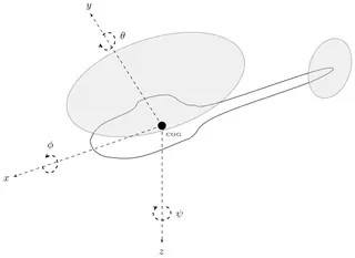
Eighteen physics figures, almost all from Janosh Riebesell’s diagrams collection. The largest group is statistical and thermal physics: the Maxwell–Boltzmann speed distribution, ideal and van der Waals isotherms, an Otto cycle on a p–V diagram, critical temperature curves, spontaneous magnetisation, gas pressure on a wall and the Bose–Einstein distribution in 3D. There are also a Bloch sphere, scattering and detailed balance, Thomson scattering, four solid-state figures (a k-space lattice of states, the Seebeck effect, basis plus lattice equals crystal, a ferroelectric response), three field-theory sketches and a helicopter free-body diagram.
Seven of the figures are plots made with pgfplots, the plotting package built on TikZ. The Feynman diagram uses the TikZ-Feynman package and the Seebeck figure loads circuitikz; the others are plain TikZ with libraries such as calc, angles, quotes and decorations.markings.
Quantum & particles
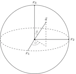
Bloch sphere
MIT licence, © Janosh Riebesell and contributors · janosh/diagrams
Open in the TikZ editor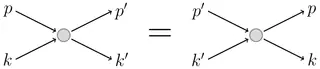
Scattering and detailed balance
MIT licence, © Janosh Riebesell and contributors · janosh/diagrams
Open in the TikZ editor
Statistical & thermal
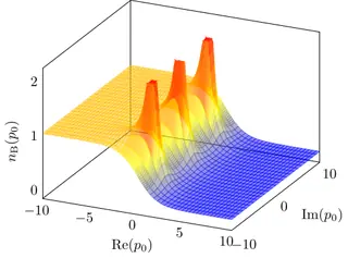
Bose–Einstein distribution (3D)
MIT licence, © Janosh Riebesell and contributors · janosh/diagrams
Open in the TikZ editor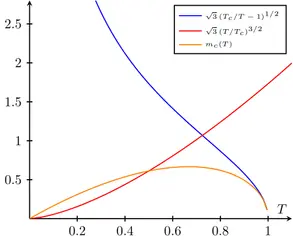
Critical temperature curves
MIT licence, © Janosh Riebesell and contributors · janosh/diagrams
Open in the TikZ editor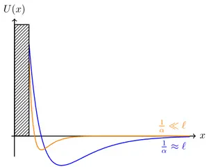
Gas pressure on a wall
MIT licence, © Janosh Riebesell and contributors · janosh/diagrams
Open in the TikZ editor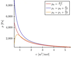
Ideal and van der Waals isotherms
MIT licence, © Janosh Riebesell and contributors · janosh/diagrams
Open in the TikZ editor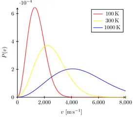
Maxwell–Boltzmann speed distribution
MIT licence, © Janosh Riebesell and contributors · janosh/diagrams
Open in the TikZ editor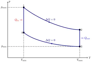
Otto cycle (p–V diagram)
MIT licence, © Janosh Riebesell and contributors · janosh/diagrams
Open in the TikZ editor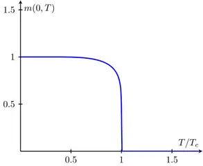
Spontaneous magnetisation
MIT licence, © Janosh Riebesell and contributors · janosh/diagrams
Open in the TikZ editor
Waves & optics
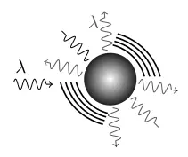
Thomson scattering
MIT licence, © Janosh Riebesell and contributors · janosh/diagrams
Open in the TikZ editor
Mechanics
Solid state & materials
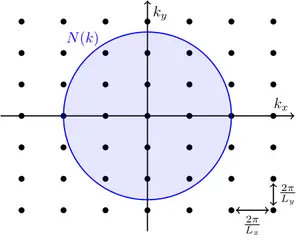
k-space lattice of states
MIT licence, © Janosh Riebesell and contributors · janosh/diagrams
Open in the TikZ editor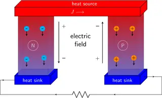
Seebeck effect (thermoelectric)
MIT licence, © Janosh Riebesell and contributors · janosh/diagrams
Open in the TikZ editor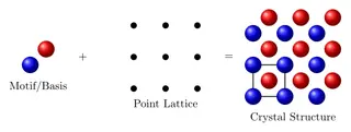
Basis plus lattice equals crystal
MIT licence, © Janosh Riebesell and contributors · janosh/diagrams
Open in the TikZ editor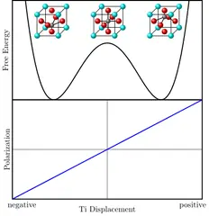
Ferroelectric response
MIT licence, © Janosh Riebesell and contributors · janosh/diagrams
Open in the TikZ editor
Field theory
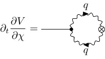
Feynman diagram with a loop
MIT licence, © Janosh Riebesell and contributors · janosh/diagrams
Open in the TikZ editor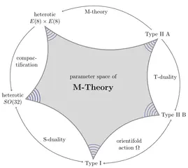
M-theory and its limits
MIT licence, © Janosh Riebesell and contributors · janosh/diagrams
Open in the TikZ editor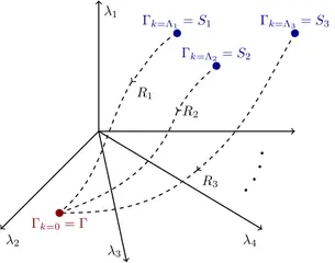
RG flow in theory space
MIT licence, © Janosh Riebesell and contributors · janosh/diagrams
Open in the TikZ editor
Using these figures
Every figure keeps its own licence: MIT or CC0 1.0, both of which allow use, change and sharing, commercial use included. The MIT licence asks that its copyright and permission notice go with copies of the code, so each figure’s code starts with its source, author and licence; keep those lines when you reuse it. The full licence texts are on the sources and licences page.
“Open in the TikZ editor” loads the figure’s complete document into the free TikZ editor, where it is typeset with TeX Live 2026 and you can change it and download a PNG. To compile it on your own computer, save the code as a .tex file and run pdfLaTeX (or the engine the tile names) on it; LabCanvas changed the files only where needed to make each one compile on its own, as its first lines say.