TikZ computer science examples
Contents
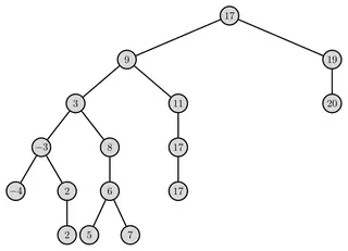
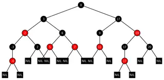
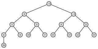
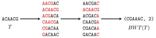
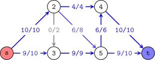
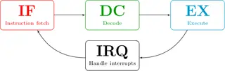
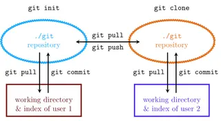
Twelve figures: four data structures (a binary search tree, a red–black tree, a binary heap and a singly linked list), three algorithms (the Burrows–Wheeler transform, a maximum flow problem and a shortest path in a weighted graph) and five systems diagrams (the fetch–decode–execute cycle, a Git workflow, the bit layout of an IEEE 754 floating-point number, a system block diagram, and virtual machines compared with containers).
The trees and lists show how TikZ handles linked structures: nodes placed with positioning or the tree syntax, multi-part nodes from shapes.multipart for list cells, and edges between named nodes.
Data structures

Algorithms
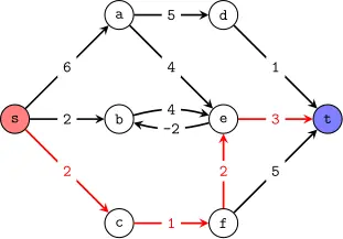
Shortest path in a weighted graph
MIT licence, © Petar Veličković · PetarV-/TikZ
Open in the TikZ editor
Systems & architecture
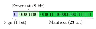
IEEE 754 floating-point number
MIT licence, © Martin Thoma · MartinThoma/LaTeX-examples
Open in the TikZ editor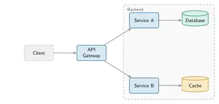
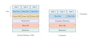
Virtual machines vs containers
MIT licence, © Andreas Bauer · andreas-bauer/tikz
Open in the TikZ editor
Using these figures
Every figure keeps its own licence: MIT or CC0 1.0, both of which allow use, change and sharing, commercial use included. The MIT licence asks that its copyright and permission notice go with copies of the code, so each figure’s code starts with its source, author and licence; keep those lines when you reuse it. The full licence texts are on the sources and licences page.
“Open in the TikZ editor” loads the figure’s complete document into the free TikZ editor, where it is typeset with TeX Live 2026 and you can change it and download a PNG. To compile it on your own computer, save the code as a .tex file and run pdfLaTeX (or the engine the tile names) on it; LabCanvas changed the files only where needed to make each one compile on its own, as its first lines say.